
Chapter 28 of Naval Ordnance and Gunnery, Volume 2 — Fire Control covers antisubmarine warfare (ASW) — the detection, tracking, and attack of submerged enemy submarines by surface antisubmarine (A/S) ships. The chapter treats the equipment actually used rather than the tactical aspects of these operations. Consolidated here from the original scanned sub-pages into one illustrated, scrollable page, it covers the general nature of the antisubmarine problem and the limitations of sonar, the QHBa scanning sonar equipment, the control of the attack with the tactical range recorder and the antisubmarine attack plotter, the OKA-1 sonar-resolving equipment, and the depth-determining sonar equipment.
Note on notation: this chapter uses the book’s symbols — Rq sonar range, Bq true sonar bearing, Brq relative sonar bearing, Eq sonar depression angle, cEtq computed target depression, Hq target depth, Rhq horizontal sonar range, cRhq generated horizontal sonar range, So own ship’s speed of attack, cCo own-ship course order, Tg dead time, Tf time of flight, Td sinking time, Tud time remaining until drop/fire, Re effective range of the throwing weapons, P1 the parallax base line, and V the speed of sound in water.
A. General
28A1. Introduction
Antisubmarine warfare (ASW) consists of all measures and operations directed against enemy submarines, their operating bases, and their supporting activities. Its purpose is to deprive an enemy of the effective use of his submarines. Various types of antisubmarine operations are employed in fulfilling this purpose — some offensive in nature, some defensive. The principal ones (i.e., bombing and mining, hunter-killer, escort of convoy, harbor defense, and submarine antisubmarine operations) are discussed elsewhere in this text.
In this chapter, only those operations that involve surface antisubmarine (A/S) ships will be considered. The emphasis will be on the equipment actually used to detect, track, and destroy submerged enemy submarines rather than on the tactical aspects of these operations.
Because of recent advances in the design of submarines, the newer submarines can remain submerged for long periods of time, and can operate at high speeds while submerged. These advances in submarine performance have stimulated research and development in all fields of ASW, and have made the surface A/S ship increasingly important.
It was demonstrated during World War II, and has been confirmed by operational evaluation since that time, that the air-surface, hunter-killer team is one of the most effective units in combating submarines directly. Aircraft are able to search large areas quickly, locate submarines, and attack them with rockets, machine guns, and depth bombs. Aircraft, however, are limited in their staying power and in their ability to maintain contact and attack once the submarine has submerged. It is at this point that the importance of surface A/S ships becomes apparent. With the submarine submerged, these ships can conduct a more effective search than aircraft because they carry sonar equipment. This equipment, to date, has proved to be the most effective means of maintaining contact with and hence controlling the attack on a submerged submarine.
28A2. Weapons
The various weapons used against submarines were discussed in chapter 14. Some of these are passive in nature and present no fire control problem. In this category are mines, and — though strictly speaking not weapons — nets and booms. Other weapons effective against surfaced submarines do not present a control problem substantially different from any other surface fire control problem. This is true in the use of guns and torpedoes of surface ships, and very nearly true of all aircraft and submarine weapons when used against submarines.
The primary antisubmarine weapons of surface vessels are depth charges and hedgehogs. Rockets and torpedoes are becoming increasingly important as antisubmarine weapons, but a discussion of their application is beyond the scope of this chapter.
28A3. Underwater detection
A/S ships use echo-ranging equipment to determine the range and bearing of submerged submarines. Echo-ranging equipment is used to a lesser extent for navigation. In pilot waters, especially when visibility is low, it may be used to locate reefs, other submerged objects, and buoys. Echo-ranging equipment is commonly referred to as sonar, a name derived from its long title: SOund NAvigation And Ranging.
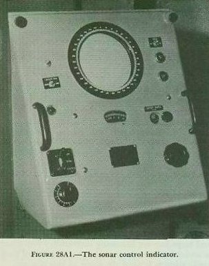
Sonar equipment makes use of ultrasonic (above audibility) sound waves. When a sound wave, traveling through water, strikes a submerged or partially submerged object, a part of its energy is reflected, and returns to its source as an echo. Sonar equipment projects sound waves into the water, and receives their echoes, by means of a submerged transducer located forward and near the keel of the A/S vessel. The signal-receiving and indicating equipment (the so-called stack or sonar control indicator) is located in a space known as sonar control. The sonar control indicator is shown in figure 28A1. The signal-transmitting equipment, which requires no operator, is usually installed in a space immediately above the transducer.
The principal sonars in use during World War II projected a narrow beam of sound into the water, and target indications were returned as audio responses from a speaker or headset. A thorough search was a slow process in that the operator hand-trained the transducer in increments of 2° to 5°, according to search doctrine in force.
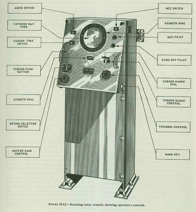
At the close of World War II, the Navy perfected a new type of search sonar known as scanning or azimuth search sonar (fig. 28A2). With each outgoing burst of sound, azimuth sonar searches through 360°, less a narrow sector allowed for the ship’s baffles. In addition, scanning sonar offers both video and audio presentation of target information.
28A4. Limitations of sonar
The behavior of sound waves in sea water is a complex study in itself. But an understanding of sonar equipment and its operation requires a general knowledge of the principles of underwater sound. The usefulness of sonar is limited by three factors:
1. Variations in the speed of sound. Under standard conditions of temperature (36°F), pressure, and salinity, the speed of sound in sea water is 4,800 feet per second. An increase in water density results in an increase in the speed of sound. An increase in pressure or salinity, or a decrease in temperature, will cause a small increase in density. (Because sea water is nearly incompressible, the effect of pressure is very slight.) Temperature has another, more important effect. Since an increase in temperature causes an increase in molecular activity, it produces a relatively large increase in the speed of sound. Thus the speed of sound will increase when the water temperature rises, even though the density of the water is decreased.
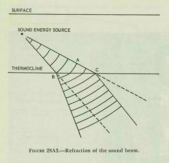
2. Refraction of the sound beam. Variations in the speed of sound (primarily due to temperature variations) result in refraction (bending) of the sound beam, as shown in figure 28A3. The upper layer of sea water is usually of fairly uniform temperature. At the bottom of this layer is a thermocline — a thin layer with a high thermal gradient (that is, a relatively abrupt change in temperature). The depth of the first thermocline, known as the layer depth, is usually between 50 and 100 feet. Below the thermocline, the temperature is again fairly uniform, but lower than in the surface layer. Figure 28A3 shows how a sound beam, striking a thermocline at any angle other than a right angle, will be refracted downward. The sound wave striking the thermocline at point B slows down, while point A on the same sound wave continues at the original speed until it strikes the thermocline at C. As a result, the wave fronts become more nearly horizontal. Because the sound beam moves in a direction at right angles to the wave fronts, it bends downward. (This effect is very similar to the refraction of light, explained in chapter 16.)
Refraction of the sound beam at the thermocline has three important effects: (1) It reduces the range at which submerged objects can be detected. Because of temperature irregularities in the thermocline, a part of the sound energy that strikes it will be scattered and lost. A part of the returning echo will be lost for the same reason. (2) It causes errors in measurement of target depth. Because the sound beam bends after it leaves the transducer, and the echo beam bends before it returns to the transducer, any measurement based on depression of the sound beam will be in error. (3) It causes errors in measurement of target range. Because the sound beam does not travel in a straight line, the actual range of the target will be less than the measured range. Errors in range measurement are usually much smaller than errors in depth measurement.
3. Echoes. The sonar transducer may receive both single echoes and reverberations (multiple echoes) from marine life, the sea bottom, surface waves, and other irregularities in the water. These echoes and reverberations tend to obscure the echo from the target submarine.
Although adverse water conditions may limit the effective range of sonar, and make it difficult to determine the exact bearing of a contact, A/S personnel are trained to get optimum results from their equipment under all conditions. They are trained to predict sound behavior and to apply the results reliably to the antisubmarine problem. Sonarmen quickly classify a contact by its appearance on the cathode-ray scope, the bearing spread and relative motion of the contact, and the quality of the echo sound. Sonar research has established certain sound “patterns,” based principally on underwater temperatures. With the aid of the bathythermograph, a device for measuring water temperatures down to 1,000 feet, it is possible to predict the sound pattern and to introduce appropriate data into the sonar system.
28A5. Antisubmarine fire control problem
The antisubmarine attack problem is similar to the surface fire control problem in that the attacking ship is considered to be moving in a horizontal plane and relative rates are computed in this plane. Antisubmarine weapons for attacking a submerged target do not have the flexibility of deck guns. Instead of computing gun orders, it is necessary to compute the course and time-to-fire in such a manner that the depth charges or throwing weapons will arrive at the predicted target position (including depth) when the submarine does.
Depth charges are either rolled off the stern of the attacking ship or projected a fixed small distance to the side. Throwing weapons are projected to a position either fixed in relation to the attacking ship or controllable within narrow limits. The fire control problem is largely a tactical problem for this reason. It is not possible to solve this fire control problem in terms of projecting the missile from any location of the ship to the target: instead, it is necessary to solve the problem of how to conn the ship into attack position.
In the case of depth charges this attack position is ahead of the submarine, to allow for the sinking time of the depth charges. How far ahead is a major variable quantity which depends on the depth of the target, the sinking speed of the charges, and the target course and speed.
For throwing weapons, the tactics differ. There is no necessity for passing ahead of the submarine, since the missiles are projected ahead to fall at the indicated position of the target. Sinking time is less for these missiles than for depth charges, but there is time-of-flight to be considered also. The other variables exist, but must be so calculated as to bring the target to a position off the attacking ship’s bow.
The projection of throwing weapons has two great advantages over the dropping of depth charges. First, in a depth charge attack, the attacking ship must pass over or nearly over the submarine to reach its attack position, and it usually loses sonar contact when it does so. It is not necessary to pass over the target to reach position for a throwing attack. Second, hydrostatic depth charges explode whether close to the target or not, and the explosion causes a disturbance of the water which interferes with sonar; throwing weapons explode on contact only, so misses do not interrupt sonar contact. (This second advantage is being offset by increased use of influence-type depth charges such as the Mark 14.)
Depth charges may be dropped from the racks at the stern, or fired from side throwers (K-guns) which hurl them as far as 125 yards on the beam. Ships lacking side throwers, of course, can drop charges only along a straight line; but if K-guns are installed any one of several standard patterns may be fired. The type of pattern depends upon the situation and the number of throwers.
While the attack is always calculated with reference to one charge — the center one of the pattern — the extensive possibility of an error makes the use of additional charges necessary. Therefore they are ordinarily dropped in patterns. When hydrostatic charges are employed, they are set to explode at various depths in the water beneath the surface area covered by the pattern.
Explosives fired under water can do greater damage than a corresponding amount of explosive set off in the air. Nevertheless, modern submarines are so strong that a charge must explode close aboard to have conclusively destructive effect.
Explosions beyond the lethal range may indirectly cause destruction of the submarine through leaks in the hull, jamming of the hydroplanes, or other forms of damage.
There are two major types of depth charge attack, known as urgent and deliberate. The urgent attack is made to harass the sub and prevent accurate torpedo fire. It consists of a pattern of one or more charges fired immediately, with shallow settings, in an attempt to drive the submarine down and prevent it from firing torpedoes. In an urgent attack, only hydrostatic charges are used.
The purpose of a deliberate attack is to destroy the submarine. A pattern is dropped in such a way that the center charge of the pattern will explode against the submarine. The pattern used for a deliberate attack is the standard full pattern of charges fired by the attacking vessel.
The chief difficulty with any attack is the time required for the charges to sink. The obsolescent 750-pound depth charge, for example, requires about 40 seconds to reach a depth of 250 feet. During this time the submarine can maneuver without interference. In 40 seconds an 8-knot submarine can travel 180 yards, make a 60° turn, and even change its depth by 60 feet.
There is a repetition of the situation encountered in gunfire. Unless the submarine is stationary, the charges can no more be dropped directly over it than a gun can be fired directly at a moving target and score a hit.
If the sub is moving straight along the attacking ship’s path, it is a simple matter to compensate for the sinking time of the charges. If the attacking ship is approaching the sub head-on, it may drop the charges before passing over the sub.
In both direct bow and stern attacks, the submarine commander has a good chance to evade the attacking ship — and he will, if possible. Sonarmen aboard the sub can hear the attacking ship, and the submarine will rarely move along the ship’s track.
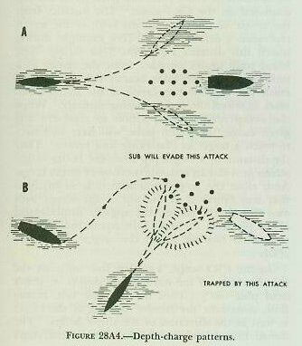
If a pattern were laid as shown in part A of figure 28A4, the sub could evade by turning in either direction. The antisubmarine vessel, therefore, must counter the sub’s evasive tactics by a maneuver similar to the one shown in part B of figure 28A4. Even though the sub tries to turn, it will come in contact with one of the charges of the pattern.
When sonar contact is made and direction of target movement is established, the antisubmarine ship is brought to a course which will take it across the bow of the submarine and sufficiently far ahead to allow for the sinking time of the charges. Thus the depth charges will explode at the same time the sub reaches them.
In order to steer the proper course, the conning officer must know the range and also the approximate bearing, course, speed, and depth of the sub. Even with all this information, the attack course selected is subject to change at any moment because of the sub’s maneuvers. Unfortunately these maneuvers may go undetected. At very short ranges, 150 yards or less, the return echo of the sonar equipment cannot be distinguished from the outgoing signal. Also, contact may be lost at longer ranges; for example, contact may be lost at 700 yards if the sub is deep enough. Thus the sub’s position will often not be known exactly in the last stages of the attack.
To reduce both the length of this “silent period” and the chances of evasion by the sub, the surface vessel generally attacks at as high a speed as possible. (The conning officer must also make certain that his ship will clear the explosions of the stern-dropped charges.) The maximum attack speed, however, is limited. At high speeds the water noises caused by the sonar transducer traveling through the water may obscure the sound echoes from the sub.
28A6. Throwing weapons
During an attack with throwing weapons, the sonar operator must hold contact with the sub and furnish the conning officer with continuous ranges and bearings. The conning officer then keeps the ship headed toward the estimated future target position and comes in for the attack. Because the charges have a fixed range, the pattern must be fired when the ship reaches the correct firing range. The correct firing range depends upon many factors, most of which are calculated in advance and set into the range recorder, attack plotter, and OKA equipments.
28A7. Conclusion
Other types of weapons and other forms of attack are under development, but their security classification is such that they cannot be considered in this text.
B. QHBa Scanning Sonar Equipment
28B1. QHBa scanning sonar equipment — general
At the present time, sonar equipment model QHBa is in use on some of the operational destroyers, and at most training activities. Although this will be the only equipment described in this text, it is now being replaced in the Fleet by model SQS-4 and related equipment. This model differs from the QHBa in details of construction and circuitry, but not in general principles.
Model QHBa combines echo-ranging and listening equipment in one unit. On a cathode-ray tube (CRT) scope, similar to a radar PPI-scope, it provides a continuous visual display of echo reception from all directions in azimuth, and an audible response from any desired single direction.
The QHBa equipment consists of the following five major units:
1. Indicator control.
2. Transmitter-receiver.
3. Transducer.
4. Scanning switch assembly.
5. Data converter.
These units, their functions, and their operation will be discussed in detail in the articles following.
28B2. QHBa indicator control
The QHBa indicator control, as its name implies, controls the operation of the QHBa equipment and provides for the video and audio presentation of target echoes.
1. Video presentation. At the instant that a pulse of sound energy is projected into the water in all directions, a luminous spot on the CRT scope (i.e., the trace of the electron beam) begins to spiral outward from the center. This spiraling motion is in reality a combination of two motions. One, a straight-line movement of the spot toward the periphery of the scope, is called the linear sweep. The other, a circular movement of the spot about the center of the scope, is known as the circular sweep. The linear sweep occurs at a relatively slow rate of speed. The circular sweep, on the other hand, occurs at a relatively high angular rate (1750 rpm). The result is that the QHBa operator observes the motion of the electron beam trace or spot not as a spiral but rather as an expanding circle of constantly increasing radius.
When the outgoing pulse of sound energy strikes a submerged object such as a submarine, part of its energy is reflected as a target echo. This echo, after being received, changed into an electrical signal, amplified, and rectified, is applied to the control grid of the cathode-ray tube and causes a bright spot or pip on the CRT-scope. Because of the persistence of the scope, this pip, along with other target pips, remains on the scope long enough to be reinforced by another returning echo. The result is a map-like presentation which is invaluable in target detection.
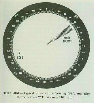
The range and bearing of a sonar contact can be determined easily from the position of the pip displayed on the CRT-scope. The distance from the center of the CRT to the edge of the screen represents a definite range. (For example, during search this distance represents 3750 yards.) The beam trace moves outward from the center at a uniform speed, and takes exactly twice as long to reach the edge of the screen as the sound pulse takes to travel the corresponding distance. When the sweep reaches the position to represent any given range, the sound pulse will have had time to reach a target at that range and return. Thus the distance of a target pip from the center of the screen provides an accurate measure of target range. And, since the scope presentation is so oriented that true North is at the top of the screen with own ship at the center, the angular displacement of the pip from the top of the screen indicates the true sonar bearing Bq of the target. See figure 28B1.
On the CRT-scope, a dotted line indicates the true direction of the stern of the ship (i.e., ship’s head plus 180°). Thus the operator can, at any time, determine the relative bearing of the target as well as the direction of the ship’s baffles. The dotted line extends in the direction of the ship’s stern, rather than its bow, so as not to obscure the target pip during an attack.
2. Audio presentation. The audio scan covers eleven degrees of bearing. It is controlled by the bearing knob, which is discussed in a subsequent paragraph. The direction of the audio scan (i.e., the direction in which the QHBa equipment is trained to receive an echo) is indicated on the CRT scope of the QHBa indicator control by a bright line called a cursor. The cursor flashes on the scope at the instant the outgoing sound pulse is transmitted. Its length is adjustable. When the cursor bisects the target pip, and its length is so adjusted that its outer end just touches the pip, the cursor bearing will be the true sonar bearing Bq, and the cursor length will furnish an indication of sonar range Rq.
The returning echo, after conversion to an electrical signal and amplification, is changed to an audible frequency and sent to a loudspeaker near the QHBa indicator control, where it is heard as a sharp “ping.” This ping is of value in target identification, and in the determination of doppler.
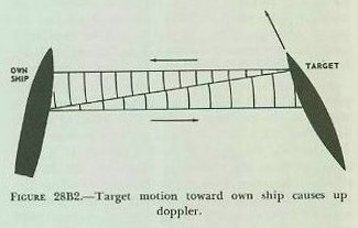
Up doppler results from an increase in frequency, or pitch, of the returning sound waves, caused by a target’s true motion toward own ship. Down doppler results from a decrease in frequency of the returning sound waves, caused by a target’s true motion away from own ship. A target that causes up doppler is said to have bow aspect, while a target that causes down doppler has a stern aspect. In other words, target motion or aspect (but not range rate) can be deduced from the doppler effect. To determine doppler, the sonarman must compare the pitch of two echoes; the first echo, consisting of reverberations from the water immediately surrounding the transducer, is compared with the echo that returns from the submarine. The relative frequency of the target echo depends on whether the submarine compresses the sound wave (up doppler, indicating bow aspect), expands it (down doppler, indicating stern aspect), or sends it back unchanged (no doppler, indicating beam aspect). See figure 28B2.
Own ship’s motion affects the pitch of the initial echo; but since it has the same effect on the pitch of the returning target echo, the doppler detected by comparison of the two is not changed by own ship’s motion, and it is this comparison that indicates the target aspect.
To facilitate the detection of doppler, doppler nullifier circuits are installed in the QHBa. These circuits remove the effect of own ship’s motion on the pitch of the echoes heard by the sonarman. In this way the variations caused by changes in own-ship speed and course are eliminated, making doppler detection easier.
3. Controls. Figure 28A2 shows the various knobs, switches, etc., on the control panel of the QHBa indicator control. Collectively, they are used to operate all the scanning sonar equipment.
a. Bearing knob and bearing dial. The true bearing of the cursor (and hence of the audio scan) is controlled by the bearing knob and is indicated on the bearing dial. The knob, when turned, will change the cursor bearing at a relatively slow rate. However, if the knob is pressed in and rotated one-eighth of a revolution in either direction, the cursor will slew rapidly. As explained previously, if the cursor is positioned so that it bisects a target pip, the cursor’s bearing will be the true sonar bearing Bq of that particular target. Bq can be read on the bearing dial.
b. Range knob and range dial. It was noted above that the length of the cursor (and hence cursor range) could be varied. The range knob is the control which determines this length. It is located directly above the bearing knob and has adjacent to it a range dial on which approximate values of cursor range can be read. Again, if the outer tip of the cursor just touches a target pip, the value of range indicated on the range dial will be an approximate value of sonar range Rq to that particular target. Such a value, of course, is of interest only when making an initial contact report. Accurate values of Rq, as will be explained later, are determined by the OKA-1 range recorder for use in the antisubmarine fire control problem.
c. Keying selector switch. This switch has three positions: 1500, 3750, and LISTEN. When it is moved to the position marked 3750 (during search and when tracking a target at a range greater than 1500 yards), the scale of the CRT-scope (i.e., the distance from the center of the scope to the periphery) becomes 3750 yards. Similarly, when the keying selector switch is moved to the position marked 1500 (when tracking a target within 1500 yards), the scale of the scope becomes 1500 yards. In each of these cases, the video sweep (i.e., the expanding circle) moves all the way out to the periphery of the CRT-scope before collapsing and starting anew from the center. Thus it can be seen that the keying selector switch controls not only the range scale of the CRT-scope but also the time between successive sweeps. Finally, when the keying selector switch is set on LISTEN, automatic sound-pulse transmission is stopped, underwater signaling by means of a hand key is possible, and the direction of ultrasonic-frequency noise sources can be determined by observing the bearing of radial patterns on the CRT-scope which represent acoustic signals from those sources.
In this position the expanding circular sweep is still sweeping across the face of the scope at a keying interval corresponding to 3,750 yards, although no sound beam is being transmitted. Any noise of sufficient volume and appropriate frequency is picked up by the transducer and displayed on the CRT-scope as a pie-shaped brightened area. The bearing of the noise source can be determined by positioning the cursor through the middle of the brightened sector. The range can not be determined, since the scope is saturated with noise.
d. Cursor push button and cursor time switch. These controls determine the duration of cursor illumination. The cursor push button is pressed whenever it is desired to have the cursor remain lighted on the CRT-scope (in order to determine accurately the bearing of a target, for example). The cursor time switch is used to control the duration of the cursor “flash”; if moved to the SHORT position (the normal position during search), the cursor will appear only momentarily when the video sweep begins to move out from the center of the CRT-scope; if the switch is moved to the LONG position (the normal position during attack), the cursor will remain on during the scan period until shortly before the echo is expected to appear (until the video sweep is 200–300 yards short of the pip position).
e. Other controls and indicators. The GAIN control adjusts the gain of both the video reception (the pip) and the audio reception (the ping) simultaneously. The AUDIO switch enables the operator to improve the signal-to-noise ratio (and hence the sharpness of the pip) whenever a noisy target is encountered. The MCC switch (an ON-OFF switch) is used for maintenance of close contact; that is, when moved to the ON position it causes the sound beam to be broadened vertically to permit tracking of targets at closer ranges. The MCC pilot light becomes lighted whenever the MCC switch is on. The GYRO OFF pilot light, when illuminated, indicates that the top of the CRT-scope represents own ship’s bow rather than true North, because of a gyro failure.
The mark signal switch and the aided tracking switch, located on the left and right sides of the control panel, respectively, are used in conjunction with the attack director and therefore will not be described here.
28B3. QHBa transmitter-receiver
At the instant the video sweep begins to move outward from the center of the CRT-scope, the keying circuits of the QHBa indicator control send a signal known as the keying pulse to the QHBa transmitter-receiver. The pulse initiates operation of the transmitting circuits in the latter unit. The transmitting circuits, in turn, produce a high-voltage pulse of electrical energy at a proper supersonic frequency (about 25.5 kc) and transmit this pulse via the scanning-switch assembly to the transducer.
Returning echo signals from the transducer, on the other hand, after passing through the scanning switch assembly, come to the receiver circuits of the QHBa transmitter-receiver, where they are amplified to a suitable level for audio and video presentation. The video signals, moreover, are rectified in order that they may be applied directly to the control grid of the CRT-scope in the QHBa indicator control for screen brightening. And the frequency of the audio signal is changed to a sonic or audible frequency, so that it may be heard over the loudspeaker used in conjunction with the QHBa indicator control.
28B4. QHBa transducer
This unit is mounted in a sound dome below the hull of the ship. Its functions, briefly, are —
1. To convert the pulse of electrical energy received from the transmitter-receiver into a pulse of acoustic energy of the same frequency, and to project this pulse into the surrounding water in all directions in azimuth.
2. To receive the returning echoes and to convert them into electrical energy of the same frequency.
These functions, it can be seen, are similar to those performed by the antenna of a radar.
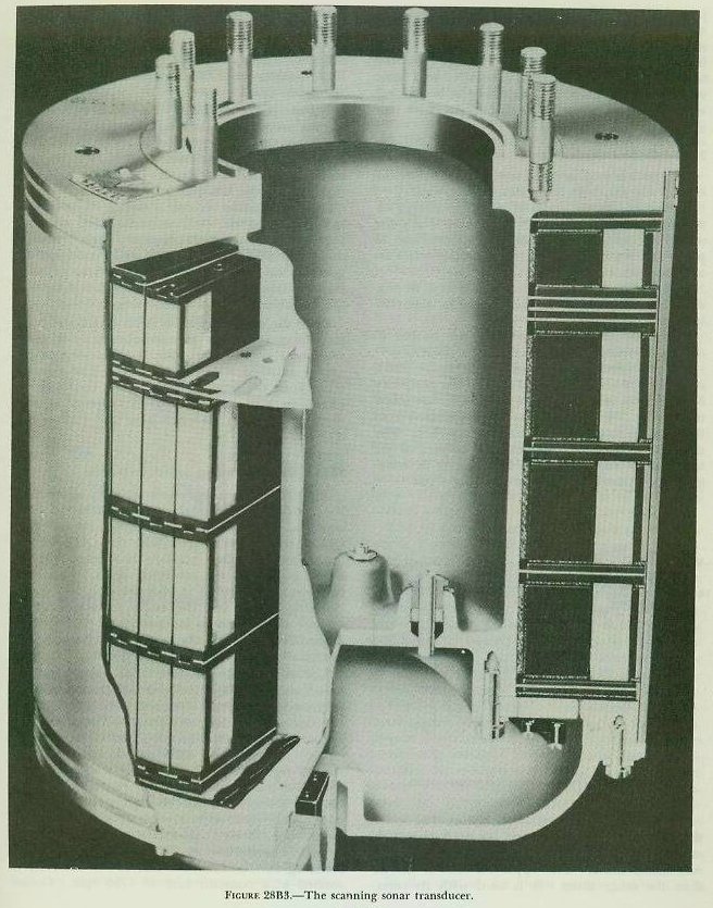
The transducer proper, shown in figure 28B3, consists of 48 staves mounted around the periphery of a circle in much the same manner as the staves of a barrel. The staves, in turn, are separated from the surrounding water by a rubber jacket. The density of this jacket is the same as that of sea water; thus any vibration of the staves is transmitted unaltered into the surrounding water.
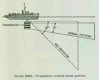
Each stave consists of four elements. The lower three are of the same size, and are used with their counterparts in the other staves to form the normal sound beam. The upper element is shorter than the other three. It is used with its corresponding elements in the other staves to form a beam which is broadened vertically and which, consequently, is desirable for the maintenance of close contact. The upper elements are used when the MCC (maintenance of close contact) switch is on. See figure 28B4.
All the staves are made of a nickel alloy which has the property of vibrating whenever an alternating magnetic flux penetrates it. This property is known as magnetostriction. Each element of a stave is surrounded by a coil. During transmission, this coil receives an alternating current from the QHBa transmitter-receiver. When this current passes through the coil, an alternating magnetic field is produced which penetrates the element of the stave, causing it to vibrate and hence produce a sound wave. The magnetic field is so adjusted that the frequency of this vibration is the same as the frequency of the applied current.
Once the sound pulse has been transmitted, the transducer staves act as microphones; and, upon receipt of a returning echo, the sequence of the events outlined above is reversed. The acoustic echo causes the staves to vibrate; and the vibrating staves, in turn, cause electrical currents to flow through the coils and hence to the transmitter-receiver.
28B5. QHBa scanning-switch assembly
The QHBa scanning-switch assembly determines the bearings of returning echoes and hence of sonar contacts. It is installed electrically between the QHBa transmitter-receiver and the QHBa transducer, and therefore controls both the outgoing sound pulse and the returning echo. There are two scanning switches in this assembly, the video scanning switch and the audio scanning switch, each of which operates independently of the other. Essentially both are the same, mechanically and electrically.
1. Video scanning switch. The video scanning switch consists basically of two metalized glass discs separated by a narrow air space. One disc is called the stator; the other, the rotor. The rotor and stator have 48 aluminum capacitor segments each, equally spaced about their peripheries. Each of the 48 segments of the stator is connected electrically to a corresponding stave of the transducer. On the rotor, 30 of the 48 segments are shorted out so that, in effect, there are only 18 active segments (i.e., 18 segments that can receive electrical signals from the stator). The stator of the video scanning switch is fixed. The rotor, however, is rotated at a constant rate of 1750 rpm. Consequently, target echo signals received from the 48 staves of the transducer by the 48 segments of the stator can be scanned consecutively, 18 at a time, by the rapidly rotating 18 active segments of the rotor. The scanning provides video indication of the sonar bearings of all targets within 360° arc in azimuth (as will be explained below).
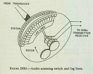
2. Audio scanning switch. This switch has essentially the same construction as the video scanning switch. However, its rotor, instead of being rotated continuously, is positioned in any desired direction by the bearing knob of the QHBa indicator control. Hence the 18 active segments of this rotor will scan echo signals from only 18 stator segments (and hence 18 transducer staves) when positioned in any one desired direction. This scanning provides an audio indication of the sonar bearing of any one particular target. Figure 28B5 is a diagram of the audio scanning switch and the lag lines (which are explained below).
3. Bearing determination. If the QHBa scanning sonar equipment were to employ a plane transducer (i.e., one with a flat transmitting/receiving surface) instead of its cylindrical one, this plane transducer would be able to transmit a sound pulse in (and hence receive a returning echo from) only one particular direction at any one time. The sonar bearing of the target echo in such a case, consequently, could readily be ascertained by noting the direction in which the transducer was trained. However, echo-ranging with such a transducer would be a slow process, hardly adequate for effective 360° search. Therefore the QHBa employs the cylindrical type of transducer described earlier in this article. This cylindrical type not only can transmit a sound pulse in every direction in azimuth simultaneously, but it can receive returning target echoes from any direction at any time between transmissions. This naturally makes possible the early detection of all targets within sonar range. Since the receiving transducer surface is cylindrical, and hence nondirectional, the direction from which a target echo is received cannot be measured by some simple method such as training the transducer itself. The video and audio scanning switches are used for this purpose.
Whenever a sound wave strikes a submerged submarine, part of its energy is reflected as an echo. This echo, upon leaving the target, fans out in several directions at once. By the time it arrives at the transducer it has, for all practical purposes, a plane front (i.e., a straight leading edge). The transducer stave nearest the target in bearing consequently receives an acoustic echo signal sooner than its adjacent staves. The video and audio scanning switch stator segments connected to this stave receive, as a result, electrical echo signals (suitably amplified by the preamplifiers of the scanning-switch assembly) sooner than their respective adjacent segments. Thus the reception of all electrical echo signals by the stators is comparable to the reception of all acoustic echo signals by the transducer. Consequently, for purposes of target bearing determination, only the stators need be considered.
It was pointed out previously that the sonar receiver bearings of a target could not be measured readily by a cylindrical transducer because of its curved surface and hence nondirectional characteristics.
The 18 active segments of the rotor are made to act as a plane transducer by the use of lag lines. The direction of the 18 active segments when the signal is received gives the bearing of the target. A similar set of lag lines can be found on the audio scanning-switch rotor. As the 18 active rotor segments of either the video or the audio scanning switch are positioned opposite any 18 segments of the appropriate stator, electrical charges on the stator segments jump the narrow air space to the active rotor segments and enter the lag lines.
The lag lines effectively “slow down” these electrical signals proportionally so that all the signals, despite their times of receipt, leave the lag lines at the same instant. In other words, the lag lines combine the voltages of these signals in the proper manner (by shifting them into phase with one another and by appropriate attenuation) to produce a total voltage which will be a maximum when the angular position of the rotor (i.e., the midpoint of the arc formed by the 18 active segments) corresponds to the actual direction of the target.
In the case of the audio scanning switch, this total voltage is sent to the receiver audio channel in the QHBa transmitter-receiver, where it is used to produce the audible “ping.” In the case of the video scanning switch, the total voltage is delivered to the receiver video channel in the QHBa transmitter-receiver, where it is amplified and rectified for use in the QHBa indicator control as a brightening signal. Since the circular sweep of the CRT scope in the QHBa indicator control is synchronized with and hence rotates at the same speed (1750 rpm) as the video scanning switch rotor, this brightening will occur at the correct bearing on the CRT-scope.
28B6. QHBa data converter
This unit has two functions. For one thing, it orients the visual presentation on the CRT-scope of the QHBa indicator control so that the top of the scope represents true North rather than own ship’s bow. Thus, for any target, true sonar bearing (Bq) rather than relative sonar bearing (Brq) is indicated on the scope.
The QHBa data converter performs its second function in conjunction with the stabilization computer. Together these two units stabilize (1) the visual CRT-scope presentation (by stabilizing the circular sweep), and (2) the audible loudspeaker reception (by stabilizing the training signal to the audio scanning-switch rotor). The result is that, as the ship rolls and pitches, the target pip on the CRT-scope will not shift its position, and the target ping from the loudspeaker will not be diminished in intensity because of the deck inclination. These corrections correspond to deck-tilt corrections in the gunnery system.
28B7. Keying circuit
The keying circuit controls the transmission of the sound pulse. This keying circuit may be controlled automatically by the QHBa indicator control (with the keying selector switch), or remotely by either the OKA-1 range recorder or the tactical range recorder. Whenever this circuit initiates a pulse, it accomplishes several functions almost simultaneously. These are —
1. It sends a pulse to the transmitting circuits of the transmitter-receiver which, in turn, send a high-voltage pulse of electrical energy via the scanning-switch assembly to the transducer.
2. It sends a signal to the scanning-switch assembly to operate a relay, which cuts out the receiving circuits of the transmitter-receiver during the time the outgoing pulse is being transmitted.
3. It collapses the previous video sweep from the CRT-scope and starts a new one by sending a linear sweep voltage to the sweep (synchro) generator of the video scanning switch; in the sweep generator this voltage is combined electrically with rotor rotation (1750 rpm) and returned to the CRT deflection plates as a new video (spiral) sweep.
4. It causes the cursor to flash on the CRT-scope.
5. It sends a signal to the depth recorder which starts the stylus excursion across the chart paper.
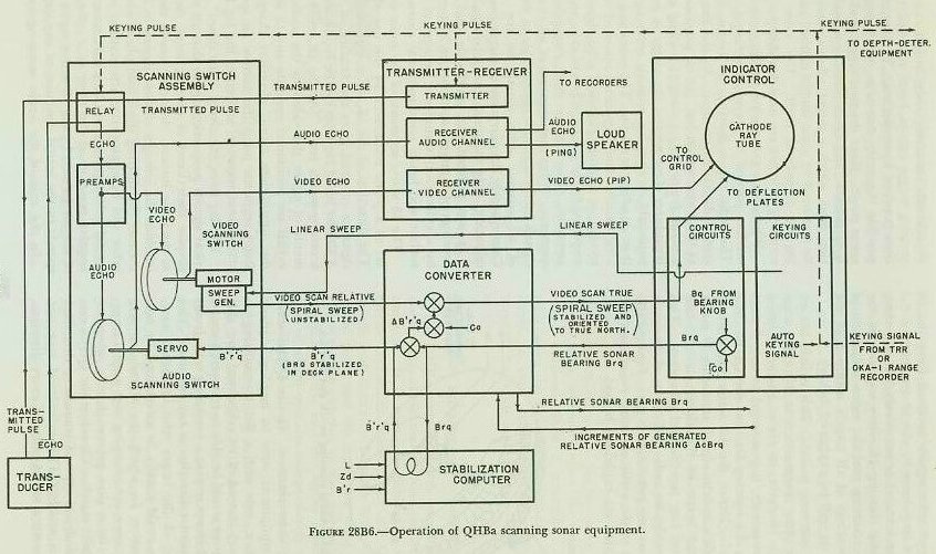
28B8. Summary
Figure 28B6 illustrates, in simplified schematic form, the operation of the various units of the QHBa scanning sonar equipment.
C. Controlling the Attack
28C1. General
Sonar can search out the target, but course to steer and firing time must be determined by other instruments. Two such instruments are the tactical range recorder (TRR) and the antisubmarine attack plotter (AP).
28C2. Tactical range recorder (TRR)
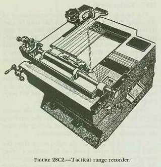
The tactical range recorder (TRR) produces a time/range plot of target echoes on chemically sensitized paper by means of a moving stylus. See figure 28C1. The stylus moves across a chart at a speed proportional to half the speed of sound in water, and the chart paper moves at a constant speed in a direction perpendicular to the stylus motion. The tactical range recorder accomplishes the following functions:
1. It provides a means for measuring sonar range Rq and sonar range rate.
2. It provides a means of determining firing time (i.e., the time when Tud = 0) for either the stern-dropped (depth-charge) attack or the throwing-weapons (hedgehog) attack.
3. It provides a visible plot of the audio reception to help identify target echoes.
4. It may be used to control the keying circuit of the QHBa scanning sonar equipment.
The TRR has two range scales. The 0–3750 range scale is etched on a black metal plate on the top of the recorder, above the window over the chart. The 0–1500 yard scale is inside the window just above the chart; it is etched on clear lucite, and illuminated by an inside light. Sonar range Rq is read by noting the appropriate scale reading of the last stylus mark made on the paper. Therefore, when on long scale, the entire width of the chart paper represents 0–3750 yards, while on short scale it represents 0–1500 yards. (Both the QHBa indicator control and the OKA-1 range recorder have the same scale arrangement.)
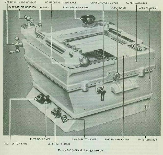
In order to measure sonar range and sonar range rate (discussed later) for both scales, using the same chart paper, it is necessary to have a range scale, stylus speed, and chart motion speed for each scale. A gear changer lever (shown in fig. 28C2) on the right side of the recorder selects the proper stylus and paper speed for each scale.
Just above the top of the chart paper is a pointer, commonly called the flyback, whose position across the chart is controlled by the flyback lever (fig. 28C2) on the front of the TRR. When the stylus reaches this flyback, it stops its recording stroke and is returned quickly to the left to start another recording excursion. The recorder sends a keying signal to the QHBa scanning sonar equipment at the instant it starts its recording motion. The position of the flyback therefore determines the keying interval of the QHBa scanning sonar equipment.
On top of the recorder is a plotter bar which is rotatable and has a lucite extension on which are etched a series of lines parallel to the plotter bar. See figure 28C3. By aligning one of these lines with the traces on the chart, the slope of the range line and hence the sonar range rate may be measured. This plotter bar is also used to determine firing time. As the range to the target closes, the traces on the plotter chart will move to the left. When the leading edge of the trace is under the firing line, it is time to fire the charge.
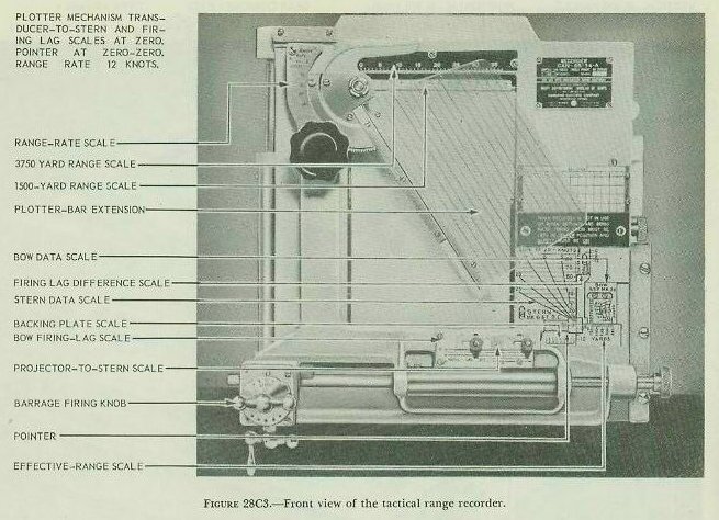
As will be seen in figure 28C3, there are several scales used to set in the various values concerned with determining the time to fire a hedgehog barrage or depth-charge pattern. The majority of these scales are set for certain physical characteristics of the ship and are not changed as the attack progresses. These are —
1. Bow firing-lag scale (inscribed FIRING LAG SEC.). On this scale is set the total time interval between the moment the A/S officer orders “Fire” and the instant the hedgehogs hit the water — dead time (Tg) plus time of flight (Tf). The dead-time factor in this setting is determined by a time study on each ship; the time-of-flight factor, from appropriate range tables.
2. Firing-lag difference scale (upper right scale inscribed 0, 6, 12). The purpose of this scale is to eliminate the necessity of changing the setting on the bow firing-lag scale every time the ship changes from a H/H to a D/C attack. The proper setting on this scale removes the error of an “earlier firing time” that would exist in a D/C attack after the bow firing-lag scale is set equal to Tf + Tg for H/H.
In order to maintain the correct time relationship between the two types of attack, it is necessary to consider the different “dead times” for H/H and D/C. If Tf + Tg (for H/H) is set on the bow firing-lag scale, it is apparent that the same value should be set on the firing-lag difference scale in order to offset the Tf + Tg which would be erroneous for D/C. At this point the setting on both scales is the equivalent of Tf + Tg for H/H equals Tf + Tg = 0 for D/C.
Since more dead time for D/C necessitates earlier firing, the stern-data scale is moved up the firing-lag difference scale a distance equal to the dead time (for D/C) from the original position (Tf + Tg for H/H). The setting for the firing-lag difference scale is therefore calculated from the formula Tf + Tg (for H/H) − Tg (for D/C).
For H/H, Tf = 8 sec.; Tg = 3 sec.
For D/C, Tg = 5 sec.
Setting on bow firing-lag scale = 8 + 3 = 11 sec.
Setting on firing-lag difference scale = 8 + 3 − 5 = 6 sec.
3. Projector-to-stern scale (inscribed PROJ. TO STERN). On this scale is set the distance in feet from the sonar transducer to the depth-charge racks on the stern (i.e., the parallax base line P1). It is obtained from ship’s plans and is constant for each ship.
4. Backing-plate scale (located beneath RE scale and inscribed FEET). The distance in feet from the sonar transducer to the depth-charge racks on the stern is set on this scale to remove the effect of the projector-to-stern scale setting when firing throwing weapons.
5. Effective-range scale (inscribed RE). On this scale is set the range of the hedgehog missiles Re as determined by the conditions existing at the time.
6. Zero-zero scale (to the left of RE scale and inscribed 0, 6, 12). This scale is used for alignment purposes.
In addition to the more or less permanent scales above, there are also two scales whose settings may have to be changed as an attack progresses. They are —
7. Stern-data scale (inscribed STERN). On this are set own ship’s speed of attack (So) and the sinking time (Td) (labeled D/C SETTING SECONDS) for depth charges. The ship’s speed is obtained from the pitometer log, and the sinking time depends on the target depth. The sinking rate for all types of depth charges has been so tabulated that the sinking time to any depth may be determined readily. Depth charges are set to explode at a pattern in depth as well as in range and deflection, in order to enclose a volume of water which will include the submarine. The measured or assumed depth which is the mean of the pattern is used in making this setting.
8. Bow-data scale (inscribed BOW). On this are set own ship’s speed of attack (So) and the sinking time (Td) for hedgehogs. As in a depth-charge attack, the ship’s speed is obtained from the pitometer log and the sinking time is calculated from the known sinking rate of the hedgehogs to the measured or assumed depth.
The settings on the stern- and bow-data scale are made by means of the data-scale indicator. This indicator is a lucite arm which is attached to the horizontal slide bar; its index, as illustrated in figure 28C3, is a “dot.” This index or “dot” is positioned over the intersection of the proper data lines (So and Td) on either the stern-data scale (for a D/C attack) or bow-data scale (for a fixed H/H attack) by means of the horizontal slide knob and vertical slide handle. As the data-scale indicator, projector-to-stern scale, bow firing-lag scale, and plotter bar are all mounted on the same frame and hence all move together whenever the horizontal slide knob or the vertical slide handle is turned, it can be seen that movement of any of the above scales will move the “dot” away from its proper position (intersection of So and Td) on the bow-data or stern-data scale or move the intersection of So and Td out from under the “dot.” The situation is then corrected by movement of the horizontal slide knob or the vertical slide handle which moves the “dot” back over the original intersection; consequently, the firing line on the plotter bar is moved closer to or farther away from the traces on the chart paper.
The manner in which a setting is made on any of the more-or-less permanent scales can be seen in figure 28C3. Briefly, a value is set on the —
1. Bow firing-lag scale, by moving the projector-to-stern scale vertically.
2. Firing-lag difference scale, by moving the stern-data scale vertically.
3. Projector-to-stern scale, by moving it horizontally.
4. Backing-plate scale, by moving the effective-range scale (RE) horizontally.
5. Effective-range scale, by moving the bow-data scale horizontally.
As previously mentioned, these settings on the more-or-less permanent scales (listed in 1–5 above) all serve to position either the stern- and bow-data scales or the data-scale indicator index with respect to the origin of the chart paper. Consequently, they either increase or decrease the time remaining until firing should occur.
For example, consider the effects of the bow firing-lag scale and firing-lag difference scale settings on firing time. From figure 28C3 it can be seen that, once the data-scale indicator index is positioned at a certain point, an increase in the bow firing-lag scale setting (a change in Tf + Tg from 9 to 12 seconds, for example) will move the data-scale indicator index down (as viewed in the illustration). Hence it will be necessary to drive the index back up to its original position by turning the vertical slide handle. Moving the index back up, in turn, will result in the plotter bar and its extension also moving up, closer to the traces, with the result that firing time for H/H will occur sooner.
Part of this motion of the plotter bar (the part corresponding to the Tf setting for H/H and any difference in Tg between H/H and D/C) will result in an incorrect firing time when firing depth charges; consequently, we must counteract this effect by setting a value on the firing-lag difference scale as explained previously. This is done physically by moving the stern-data scale until the index at the upper right corner of the scale is opposite the value of Tf + Tg (for H/H) − Tg (for D/C). This downward motion of the stern-data scale (if the index were originally at 0 seconds) will necessitate downward motion of the data-scale indicator index which, in turn, will result in the plotter bar’s being moved away from the traces, thus delaying the firing of depth charges from the point they would have been fired had this time difference between H/H and D/C not been considered. The idea of calculating settings for both the above scales can be explained from the point of convenience and efficiency, should a H/H and D/C attack be conducted on the same target. It is obvious why H/H and D/C cannot be fired at the same Tud = 0, and it is also apparent that changing the setting in seconds on the bow firing-lag scale every time you changed from H/H to D/C would accomplish the same result. Therefore, instead of continuously changing one scale, permanent settings are set on both scales making it necessary to move the data-scale indicator index only from the bow-data scale intersection of So and Td to the appropriate setting on the stern-data scale when changing from H/H to D/C attack.
Similarly, it could be shown that (1) an increased projector-to-stern scale setting would delay firing of depth charges a desired amount; (2) a corresponding increase in the backing-plate scale setting would compensate for this delay when firing fixed hedgehogs; and (3) an increased effective-range scale setting would result in an earlier firing time.
Because the tactical range recorder takes into consideration only the range aspects of the problem, the conning officer must rely on other sources for assistance in determining the proper course and speed to use to attain a firing position. Assistance from CIC, various “thumb rules” determined from experience, and a “seaman’s eye” are the general practice.
There is a barrage firing knob on the horizontal slide bar which is used to fire a pattern in range. This knob is kept in center position 3 during the approach. When the range closes to about 500 yards, it is moved to position 1, which moves the plotter bar a fixed amount to the right, thus making the firing time for the first charge of the pattern earlier than the center. When the firing line is over the leading edge of the traces, the first charge is fired and the knob shifted to position 2, which moves the firing line to the left. These steps are then repeated until all five charges have been fired.
A fixed throwing-weapons (hedgehog) attack is conducted in a similar manner, except that the bow-data scale is used and the barrage firing knob is left on position 3 (the position which corresponds to a Tud of zero).
28C3. Attack plotter
As pointed out previously, the tactical range recorder provides a means of determining the time to fire a D/C barrage or H/H pattern, based on an analysis of range and range rate data. But it makes no provision for determining the course to steer (cCo) to reach the firing position. With slow-speed submarines, the various methods of estimating this course were accurate enough to include the submarine in the D/C or H/H pattern. The advent of higher submerged speeds for submarines made necessary more precise methods for determining attack tactics. The next step in the evolution of ASW fire control equipment was the Antisubmarine Attack Plotter (ASAP) Mark 1. This instrument makes it possible to estimate more accurately the course which should be steered (cCo) to reach the desired firing position, as well as to determine the time at which firing should occur (Tud = 0). However, it was designed only for use when firing depth charges or fixed hedgehogs. It was not designed for trainable attacks. Consequently, no mention of projector train order B′gr or advance range R2 will be made in this discussion.
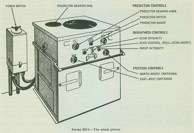
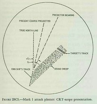
The attack plotter, shown in figure 28C4, is an electronic instrument which displays on the face of a cathode-ray tube a geographical picture of own-ship and target motion. The own-ship indication, as illustrated in figure 28C5, is a single bright dot that moves across the scope according to the true course and speed of own ship, as received automatically from the gyro compass and pitometer log. There are N-S and E-W controls on the front of the instrument for making initial settings of own ship’s position. These are similar to the controls used to position the “bug” on a Dead Reckoning Tracer (DRT). In effect, the attack plotter is an electronic DRT which shows own-ship motion automatically, as well as target position relative to own ship. The target position, which is indicated on the scope as a bright spot, is controlled by the audio section of the QHBa scanning sonar equipment. As the sound beam is projected through the water a faint line is visible on the scope, originating at own ship and proceeding in the direction the audio section is trained. If the beam strikes a target and an echo is returned, the trace is momentarily brightened so as to display on the scope a bright spot representing the target. The picture of relative motion thus presented assists the operator in determining the proper course to steer to reach the firing position.
Another feature of the attack plotter which enables the operator to better estimate the course to be steered (cCo) and the time at which to fire ahead-thrown weapons (Tud = 0) is the “predictor line.”
This is a bright line which momentarily flashes on the face of the scope immediately after own ship’s spot, and just before the sound sweep starts. The direction and length of this line can be adjusted by the operator. The true bearing of the predictor line is controlled by a predictor bearing knob on the front of the attack plotter, and read on a dial on the top. The length of the predictor line, or predictor range, is determined by a three-position knob known as the predictor switch. When this switch is in the OFF position, the predictor line does not appear on the scope; when it is set to the “1000” position, the length of the predictor line is fixed at 1,000 yards (4 inches on the scope); and when it is placed in the “RANGE” position, the length of the predictor line is governed by the three predictor range controls which, by appropriate combinations, permit the setting of any range from zero to 580 yards. Normally the predictor switch is kept on RANGE. However, the 1,000-yard position is useful on occasions when own ship and target are separated by more than the 2500-yard (10-inch) width of the scope. In such cases, own ship can be placed off the scope and still be conned toward the target by means of the long predictor line. The OFF position also is useful at times, since it permits the presentation of targets closer than 150 yards. Such targets can not normally be seen when the predictor line is shown on the scope.
In order to conduct an attack using ahead-thrown weapons, the following procedure should be used:
1. By means of the N-S and E-W controls on the front of the instrument, orient own ship and target so that the target will be headed for the center of the scope. This is done so that a continuous plot of own ship and target will be possible without the necessity of “repositioning” during the attack and thus interrupting the continuity of the plot.
2. By means of the predictor range controls, adjust the length of the predictor line to the effective range of hedgehog missiles when controlled by the attack plotter. (The computation of this effective range will be discussed in more detail later.) As previously stated, the true bearing of the predictor line may be controlled by the operator. Using the predictor bearing knob, estimate a course which when steered by own ship will result in a situation in which the end of the predictor line will pass through the predicted position of the target. It will be recalled that from the instant the word to fire is given, there will be an elapsed dead time Tg until the weapon is fired, a time of flight Tf until the pattern lands, and a sinking time interval Td until the H/H’s sink. If this total time is, for example, 20 seconds, the target will move during this 20-second period and the H/H’s must be at the predicted position at the end of this time.
The true bearing of the predictor line is automatically transmitted to an indicator on the bridge in front of the helmsman as the course to steer, or own-ship course order cCo. The target’s course can be estimated on the scope from the target’s apparent motion, and target speed can be approximated by comparison with own ship’s speed, bearing in mind that the scale of the scope is about 250 yards per inch. Continual adjustments of own-ship course order can be made as the range closes, so as to compensate for target maneuvers. The time at which firing should occur (Tud = 0) is reached at the instant the end of the predictor line leads by a proper amount the “pip” indicating the target position, or, more specifically, when it leads the target by an amount (expressed in inches) equal to target speed S times the quantity (Tg + Tf + Td). From the above it may be seen that the fire control problem is quite accurately solved from the range standpoint, but leaves much to be desired as regards determining the proper approach course. The accuracy of the proper approach course is largely dependent on the operator’s understanding of the relative motion of own ship and target.
In conducting a depth charge attack, the same general principles are used to arrive at the firing position. In this case own ship must cross over the predicted target position before the charges are dropped. In figuring the predicted position, only dead time and sinking time are used; time of flight is not considered. However, when arriving near the firing point, control is usually shifted to the tactical range recorder for firing the depth charge pattern.
D. OKA-1 Sonar-Resolving Equipment
28D1. Introduction
The OKA-1 sonar-resolving equipment consists of the following three major units:
1. Range recorder.
2. Range computer.
3. Horizontal range recorder.
Either the TRR or the OKA-1 range recorder can be used with the QHBa scanning sonar equipment to provide the keying pulse.
28D2. OKA-1 range recorder
Figure 28D1 illustrates the OKA-1 range recorder. This piece of equipment performs the following functions:
1. It records and transmits the value of sonar range Rq.
2. It provides for the measurement of sonar range rate.
3. It may be used to control the keying circuit of the QHBa scanning sonar equipment.
The recorder mechanism (as shown in fig. 28D1) is made up of a strip chart device employing moist, chemically sensitized paper which moves slowly at a constant speed in a direction perpendicular to the path of a reciprocating stylus. During its recording motion this stylus traverses the chart from left to right at a speed proportional to half the speed of sound in sea water, and is rapidly returned to the left after each stroke. The speed of the stylus is corrected for actual speed of sound conditions determined from bathythermograph readings. (See article 28E2.) This correction is set with a knob and dial on the OKA-1 range recorder. Note that this correction is not made in the QHBa.
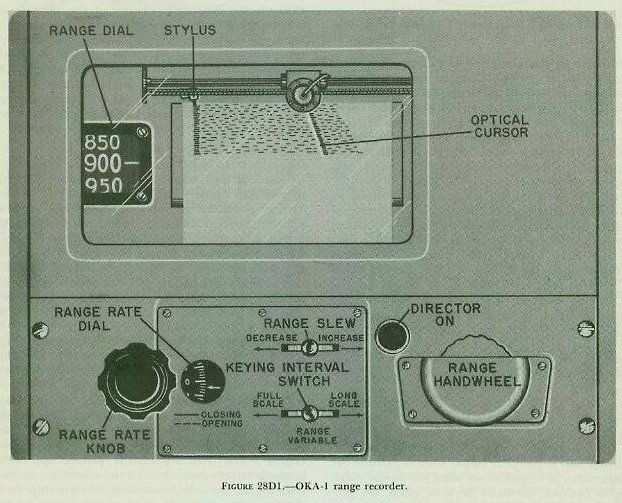
The stylus starts its recording motion at the instant the transmitted pulse leaves the transducer. The audio signal received by the QHBa equipment is applied to the stylus, causing a passage of current through the paper when an echo is received and resulting in a visible mark. Therefore, since the stylus started its motion at the instant the pulse was transmitted and moves at a rate proportional to half the speed of sound, the distance from the starting point to the mark is a measure of the sonar range to the target.
Determination of the sonar range to the target is accomplished by an optical cursor (light beam) which projects a cursor image on the recorder chart. This image is moved across the chart to the position of the last target mark by a synchro system which provides sonar range Rq to the OKA-1 range computer and, in addition, indicates the value of this range on a dial on the recorder. The optical cursor is rotatable, so that it may be lined up with a series of range marks as the paper moves down the recorder at a constant speed which represents time. The slope of the optical cursor, when properly lined up, is therefore a measure of the rate of change of sonar range.
The controls for operating the OKA-1 range recorder are located on both the top panel and the front panel of the instrument. Those on the top panel are shown in figure 28D1 and are described in the paragraphs that follow.
1. Range slew, range handwheel, range dial. The range slew and range handwheel move the optical cursor (light beam) across the scale horizontally. The slew is used to position the cursor initially on a target; the handwheel, to provide the attack director with rate control corrections. Any horizontal motion of the cursor is recorded on the range dial located at the left of the recorder chart. Whenever the cursor is properly positioned over the target, this dial indicates the instantaneous value of sonar range Rq.
2. Range-rate knob and dial. These are shown at the lower left corner of figure 28D1. The range-rate knob controls the slope of the optical cursor as well as the operation of the cursor-positioning synchro system mentioned above. When the knob is turned so that the cursor assumes a vertical position, the reading on the range-rate dial will be zero and the synchro system will not move the cursor. This is the normal condition when slewing to a new target.
However, once a target is acquired and the optical cursor is aligned with a series of range marks which collectively have a definite slope, the range-rate dial will indicate a value of range rate corresponding to that slope. Moreover, the value of range rate will cause the synchro system to position the cursor continuously over the range marks. As long as the actual range rate of the target does not change, the target will be tracked automatically and correct values of Rq will be transmitted to the OKA-1 range computer.
3. Keying-interval switch. The switch controls the keying interval of the QHBa, and thus the stylus speed and chart scale of the range recorder. This switch has three positions: LONG SCALE, FULL SCALE, and RANGE VARIABLE. In the LONG SCALE position, the chart width represents 3,750 yards and the stylus traverses the full width thereof before hitting the fixed flyback, which returns the stylus rapidly to the left. In the FULL SCALE position, the chart width represents either 3,750 yards or 1,500 yards depending upon the location of the cursor. The change of scales occurs automatically as the cursor passes about the 1,450 yard point of the scale. Thus when a target closes from say 2,500 yards to 1,450 yards, the recorder automatically shifts to the 1,500 yard scale. In the RANGE VARIABLE position, the scale selection works as in the full scale position. However, the stylus does not traverse the full width of the paper as in the other two positions but is limited to the range of the optical cursor plus 200 yards. The optical cursor carries a variable flyback which in RANGE VARIABLE operation returns the stylus to the left from a position 200 yards greater than cursor position.
28D3. OKA-1 range computer
The primary functions of this unit of the OKA-1 sonar-resolving equipment are to compute the following quantities:
1. Generated horizontal sonar range cRhq.
2. Stylus speed for the depth recorder.
To accomplish the first of these functions, the OKA-1 range computer receives inputs of sonar range Rq from the OKA-1 range recorder (as described in the preceding article) and target depth Hq from the depth recorder. With these two inputs, it then generates a value known as the computed target depression cEtq from the relationship:
Once cEtq is known through its sine function, the OKA-1 range computer can determine the horizontal sonar range from the equation:
To understand why the range computer generates horizontal sonar range in this manner, it is necessary to understand more about the refraction of the sound beam mentioned in article 28A3. If there were no refraction of the sound beam, the sonar range Rq would also be the slant range to the target; that is, the sound beam would follow a straight line connecting own ship and target, and Rq would be measured along this line. However, if the sound beam were refracted at some point in its travel by a steep temperature gradient or thermocline, Rq no longer would be the straight-line range to the target, but would be measured along the refracted sound beam. This effect is shown in figure 28D2. The target’s actual position is at point C and Rq is measured along line ABC.
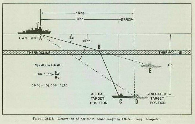
If the OKA-1 range computer were to compute horizontal sonar range cRhq from inputs of target depression Eq and a straight-line value of sonar range Rq (= ABE in the illustration), the target’s position would be established erroneously at point E. However, by generating its own value of target depression cEtq from Hq and a straight-line value of Rq (= AD in fig. 28D2), the range computer effectively establishes the target’s position as point D, which is at the correct depth and at a horizontal sonar range cRhq only slightly greater than the true horizontal sonar range Rhq. This approximation of cRhq is possible since the range error (i.e., the difference between cRhq and Rhq) progressively diminishes as the target closes and the amount of sound-beam refraction decreases.
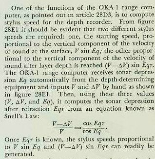
The OKA-1 range computer accomplishes its second function, the computation of stylus speed for the depth recorder, in conjunction with the depth-determining equipment. The manner in which it does this will be discussed in section E.
28D4. OKA-1 horizontal range recorder
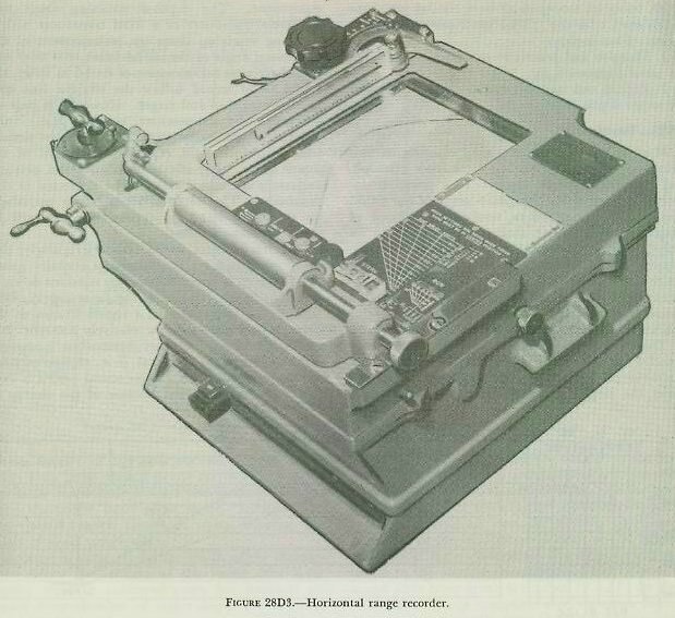
The value of horizontal sonar range cR′hq generated by the OKA-1 range computer is transmitted not only to a range and depth indicator but also to the OKA-1 horizontal range recorder (fig. 28D3) whose functions are —
1. To record the value of generated horizontal sonar range cRhq.
2. To provide for the measurement of horizontal sonar range rate.
3. To provide a means of determining firing time (i.e., when Tud = 0) for either the stern-dropped (depth-charge) attack or the throwing-weapons (hedgehog) attack.
In construction and operation, the OKA-1 horizontal range recorder is basically the same as the tactical range recorder, differing from the tactical range recorder in really only two major respects:
1. It employs a nonreciprocating rather than a reciprocating stylus.
2. Its operation is based on an input of generated horizontal sonar range cRhq rather than an input of the audio response from the QHBa equipment.
E. Depth-Determining Sonar Equipment
28E1. Introduction
No one particular type of depth-determining equipment will be described in this article. The various types employed at the present time (the QDA being an example) all have similar functions when used with the OKA-1 sonar-resolving equipment. That is, they —
1. Measure and transmit to other units the value of sonar depression Eq.
2. Record and transmit to other units the value of target depth Hq.
28E2. Description
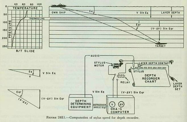
Most of the depth-determining equipments now employed in the fleet use the same basic principle for computing target depth. This principle involves measuring the depression angle of the sound beam to the target, then resolving the speed of sound in water along that sound beam into its component in a vertical plane. Then this component of the velocity of sound in water is used to control the stylus speed of a recorder, with the excursion of the stylus starting at the instant the sound is transmitted into the water and the stylus marking a recorder paper when the echo is received.
The recorder paper moves from one roller onto another, so that there will always be a new measurement of depth whenever an echo is received from the target on the depth-determining sonar equipment. The depth-determining sonar uses a tiltable transducer or a fixed transducer with a scanning receiving beam for measurement of the depression angle of the sound beam.
If there were no refraction of sound in water, the sound beam would follow the straight line connecting own ship and target. However, as pointed out previously, temperature, pressure, and salinity differences will cause variations in water density which, in turn, will result in refraction of the sound beam. The effects of salinity and pressure variations are minor and will be neglected in this discussion. The effect of temperature variations, on the other hand, is appreciable and will be discussed in more detail.
The temperature varies rather irregularly, due to currents and sea conditions. Generally speaking, however, it remains relatively constant down to a certain depth (known as the layer depth), then becomes rapidly cooler in a region known as the thermocline, and finally is relatively constant (but cooler) again until another thermocline is reached.
The effect of thermoclines (i.e., regions of steep temperature gradients) upon sound beams is twofold. In the first place, because of the change in water density at the thermocline, sound beams other than those normal to the thermocline will be refracted downward (toward the normal) as they enter the cooler, more dense water. Secondly, the speed of sound is decreased upon entering the water of lower temperature.
Because of these effects, the depth of the thermocline below the surface of the water (the layer depth) must be measured every few hours if accurate determination of target depth Hq is going to be possible. The measurement is accomplished by use of an instrument known as the bathythermograph (B/T).
The B/T, which contains pressure- and temperature-measuring devices, is lowered over the side of a surface ship on the end of a long wire. During its descent it records pressure (which is a measure of depth) versus temperature on a slide which can be placed in a viewer and read when the B/T is recovered.
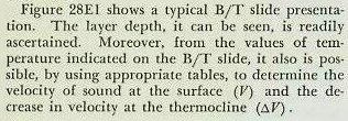
The following relationships, reproduced from the original text, govern the resolution of the speed of sound and the determination of target depth:
The change from one stylus speed to another in the depth recorder is accomplished, as shown in figure 28E1, by positioning a contact maker at a point representing layer depth. The moving stylus, upon striking this contact maker, will trip a relay in the stylus-speed circuit which will change the speed from one proportional to V sin Eq to one proportional to the quantity below:

The audio response from the depth-determining equipment is fed through the stylus in a way that marks the sensitized paper whenever a target echo is received. Basically, the operation of the depth recorder is the same as that of the OKA-1 range recorder except for the two speeds involved in stylus excursion.
28E3. Summary of the OKA-1 and depth-determining system
Figure 28E2 illustrates, in simplified schematic form, the operation of the various units of the OKA-1 sonar-resolving and depth-determining equipments.
