Naval Ordnance and Gunnery, Vol. 2
Chapter 19 — Surface Fire Control Problem

Chapter 19 of Naval Ordnance and Gunnery, Volume 2 — Fire Control presents the complete solution of the surface fire control problem. Sections progress from an analytical (mathematical) solution through graphic rangekeeping to the fully mechanical solution implemented in the Rangekeeper Mark 8, covering every basic computing mechanism and the stable vertical gyroscope system that compensates for the ship's roll and pitch.

A. General

19A1. Introduction

The fire control problem requires for its solution the collection of essential data, computations based on these data, and arbitrary correction of the results.

The Navy uses mechanical or electrical computing devices, organized into fire control systems, to perform the detailed computations. These devices provide accurate solutions to the fire control problem, with a great saving in both work and time. In a fire control system, we are more interested in saving time than in saving work. It is desirable that we solve the fire control problem correctly and deliver our weapons before the enemy can solve the problem and deliver his. Failure to do so might result in loss of the ship, and of the life of every man aboard.

The computing devices you will work with are extremely complex; you are not expected to master the details of their construction. But these machines can not think; they must be controlled by human intelligence. The solution provided by a computing device can be no more accurate than the information you put into it. To use these machines intelligently, you must have a complete understanding of their operating principles.

In general, computing devices can be divided into two broad categories:

Digital. The inputs and outputs of a digital computer are digits, and all its computations are carried out in terms of digits. The abacus is a simple digital computer that has been in use for hundreds of years. Adding machines and desk calculators are more recent examples. The principal operations performed by a digital computer are adding, subtracting, and counting.

To multiply, for example, the multiplicand is set into the computer, which is then made to add the multiplicand repeatedly, while counting the number of additions. When the number of additions equals the multiplier, the sum is the product of the multiplier and multiplicand. To divide, the dividend is set into the machine. The divisor is subtracted repeatedly from the dividend, until the number remaining is less than the divisor. The number of subtractions required is the quotient of the two machines.

Analog. The analog computer deals with continuously variable quantities, rather than with separate digits. It operates by setting up, within the machine, conditions analogous to the various factors of the problems. Thus a given quantity might be represented within the machine by a voltage, a distance, or an angle of shaft rotation. An ordinary slide rule is a simple analog computer, in which distances along the rule and the slide are analogous to numbers.

Analog computers are most useful when a given problem, represented by a given set of equations, must be solved repeatedly. This is true of the fire control problem, in which the equations remain the same although the quantities they deal with may vary. The fire control problem deals with continuously variable quantities (such as speeds and distances, and gun train and elevation angles), rather than with digital quantities. And, with an analog computer, the solution to the problem is available as soon as the inputs have been completed. For these reasons, most of the computing devices used in fire control systems are analog computers, even though some units of such systems may include certain features of digital computers.

19A2. Fire control systems

There are two broad classes of gun fire control systems:

1. Surface systems, utilizing estimated values of target course and speed and measured values of range, relative bearing and own-ship speed and course; computing necessary corrections including deck-tilt and trunnion-tilt compensation; resolving ship and target motion into linear rates; predicting the future position of the target on the basis of these rates; and computing and transmitting gun orders.

2. Dual-purpose systems, which are similar to the surface systems except that, since they fire at air as well as surface targets, they measure, in addition, target elevation as an original input.

Relative-rate method can be used with either surface or dual-purpose system, in which relative motion of own ship and target is measured by tracking the target and by using the torque generated in tracking to precess a system of gyroscopes, and modifying the gyro output by such corrections as may be necessary to obtain correct gun orders.

Angular-rate method is used with dual-purpose GFCS Mk 56.

In practice, the solution of the problem by a specific fire control system is specialized within certain limits dictated by the primary use of that system. A single-purpose surface battery system which is designed primarily for surface fire can operate on the assumption that all targets are on the surface, and it can disregard the effects of a small angle of elevation or depression of the line of sight. With this system it is perfectly possible to fire at elevated targets in shore bombardment, or even at aircraft within the elevation limits of the guns, but such action requires arbitrary corrections or interconnection with the dual-purpose computer. Since heavy machine guns are designed primarily for shooting at incoming air targets, there is no concern about the point of fall in the conventional sense, and the machine-gun fire control system can function well without some of the units which are absolutely essential to the surface or dual-purpose system. The dual-purpose fire control system limits the accuracy of its fire against surface targets, in order to be effective against aircraft and still stay within necessary limitations of space and weight.

The next few chapters are concerned with a functional explanation of the solution of the fire control problem. The surface-problem solution being simpler than that for an air target, the present chapter explores the basic nature of the surface problem and the principles required for its analytical solution. It also introduces the student to a typical array of fire control mechanisms which have been developed to perform certain of the necessary computations. In succeeding chapters, a fairly detailed investigation is made of the design and function of representative types of the three classes of fire control systems mentioned above. Definitions of terms and symbols are to be found in appendices E and F.

B. Analytical Solution

*See also chapter 17.

19B1. Steps in solving the fire control problem

The solution of the problem is to be considered in five steps:

1. Establishing present target position.

2. Computing necessary offset from the line of sight.

3. Correcting for the effects of deck inclination.

4. Computing gun orders.

5. Correcting the fall of shot.

19B2. Establishing present target position

The first step in the solution of the problem is to establish the line of sight to the target by radar or optical instruments. Accurate measurements are essential for the following:

1. Present range (R). The observed distance from ship to target, measured along the line of sight. This quantity is determined by rangefinder, by fire control radar, or if no better method is available, by estimate.

2. Relative target bearing (Br). The angle between the vertical plane through the fore-and-aft axis of own ship and the vertical plane through the line of sight, measured in a horizontal plane clockwise from the bow. Most of the computing devices used for solution of the surface problem assume that own ship and target are in the same horizontal plane. Most gun directors used with these computers, because of structural considerations, are trained in a plane parallel to the ship’s deck, so of necessity measure target bearing in this plane. Target bearing measured in the plane of the deck (B′r′, called director train) is converted to the horizontal plane by a computed correction, jB′r′, called deck-tilt correction, to become Br. B′r′ is measured with director sights or fire control radar.

If ship and target were stationary, the only corrections necessary would be those for wind and for the ballistics of the gun. However, the practical difficulty of the solution is increased by the need for computing and applying corrections for relative motion of own ship and target, and for deck inclination with respect to the horizontal.

19B3. Relative target motion

When ship and target are moving with respect to each other, gunfire, to be accurate, must compensate for the error caused by their relative motion during the time of flight of the projectile.

An appreciable time interval elapses while the projectile is in the air. This time is significant when it is considered that a ship at 30 knots is actually traveling 16.89 yards per second.

The method employed analyzes the relative motion of own ship and target to determine the rates at which range and bearing are changing, computes the amount of change during any desired time interval, and applies this change to the original measured quantity to produce continuously accurate values of the coordinates of present target position. The same rates, multiplied by the time of flight, compute the predicted change in target position during the time of flight. This procedure may be compared to the working of a clock, which, once set correctly and being so constructed that it measures the rate of the passage of time, can add increments of time to the original setting and supply us with the correct time at any later instant.

19B4. Components of relative target motion

The apparent motion of the target as seen from the deck of own ship is the resultant of the motion of both vessels. To take a simple case, if both ships are steaming down the line of sight toward each other, each at the rate of 30 knots, it is apparent that the range is closing at the rate of 60 knots. Since this is true, the component of relative target motion affecting range can be obtained by combining the range component of own-ship motion with the range component of target motion. The deflection component can be similarly handled.

In the chapter on exterior ballistics, the line-of-sight diagram was presented, with own-ship and target motion represented by vectors. The length of the vector represents speed, while the direction of the vector indicates course. The vectors were resolved into their components in and across the LOS. These components are:

Yo

Range component of own-ship velocity. The horizontal component of own-ship velocity along the line of sight.

Yt

Range component of target velocity. The horizontal component of target velocity along the LOS.

Xo

Lateral component of own-ship velocity. The horizontal component of own-ship velocity across the LOS.

Xt

Lateral component of target velocity. The horizontal component of target velocity across the LOS.

These components can be combined to provide range and bearing rates:

dR

Range rate. The time rate of change of range. The component of relative target motion along the LOS. dR = Yo + Yt.

RdBs

Linear bearing rate measured at the target. The component of relative target motion across the LOS. RdBs = Xo + Xt.

dBs

Angular bearing rate. The time rate of change of target bearing. dBs = K × RdBs/R.

K

Constant.

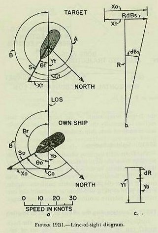
These components are illustrated in figure 19B1. The line-of-sight diagram is used to derive the components of own-ship and target motion. The direction of the effect of the components on range or bearing can best be ascertained by observation. Consider the target stationary; then examine the direction of Yo and Xo. If, as in figure 19B1, Yo causes range to increase, it is considered positive. Xo, the bearing component, is positive if, as in the figure, it causes the line of sight to move to the right (or the numerical value of bearing to increase). Then consider own ship to be motionless, and assign algebraic signs to target components by the same reasoning. In figure 19B1, by inspection, Yo and Xo are positive and Yt and Xt negative.

19B5. Range rate

In figure 19B1 (c), the range components have been added algebraically to form the range rate. Since Yt is greater than Yo and is negative, dR is negative, decreasing the range.

Range rate must be converted from knots into yards per second, since range is measured in yards. The conversion constant is the result of the following equation:

1 knot = 2,027 yards per hour / 3,600 seconds per hour = 0.563 yards per second.

19B6. Bearing rate

In figure 19B1 (b), the bearing components are added to obtain the linear bearing rate RdBs. Since Xo is positive and larger, RdBs is positive (increasing).

Since bearing is an angle, rate of change of bearing must be converted to an angular rate. RdBs is linear. The conversion is accomplished as follows:

1 knot = 0.563 yards per second.

1 yard per second = 1/R (yds) / 1000 = 1000/R (yds) mils per second.

1 mil = 3.438 minutes of arc.

1 knot at range R (yds) = 0.563 × 1000/R (yds) × 3.438 = 1936/R (yds) minutes of arc per second.

Therefore, dBs (min. of arc per sec.) = 1936 × RdBs (kts) / R (yds).

19B7. Use of range and bearing rate

Range and bearing are computed continuously by applying the rates derived in the preceding paragraphs. By continuously applying the rates it is possible to keep accurate values of present range and bearing, even though measurements of range and bearing may be interrupted. And by using time of flight, it is possible to predict the position of the target at the end of the time of flight, assuming that relative motion is constant for the short time interval involved. In practice, the error resulting from the fact that RdBs is a linear instead of an angular rate is reduced in modern computing instruments by using very short time intervals in the computation. Also for obtaining each successive instantaneous value of R and Br the new values of dR and RdBs obtained for the preceding instant are used.

This completes the analytical solution of the problem of maintaining continuous values of present and predicted range and bearing. It is immediately apparent that because of the time required for computation, the large number of calculations necessary, and the errors introduced by using finite time intervals, the analytical solution is of no practical value in modern gunnery. Mechanical and electrical rangekeepers and computers have been perfected which accomplish all the steps of the computation automatically on the basis of accurate basic inputs.

19B8. Computing bore offsets

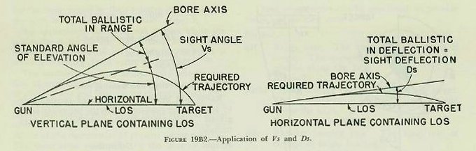
The angles by which the gun bore must be offset from the line of sight in order to hit the target are sight angle (Vs) in elevation and sight deflection (Ds) in train. Figure 19B2.

19B9. Sight angle

The chapter on exterior ballistics presented the method of determining the vertical angle by which the bore axis of the gun must be offset from the line of sight. This angle is made up of the standard angle of elevation (column 2 of the range table), plus the angular equivalent of the total ballistic correction in range, plus the angular equivalent of range spots. In fire control, this angle is called sight angle (Vs). It should be noted that one of the largest components of the range ballistic correction is normally the correction in range for relative motion of own ship and target.

19B10. Sight deflection

The horizontal angle by which the bore axis must be offset from the LOS is the angular equivalent of the total ballistic in deflection plus any deflection spots. The details of this computation were also covered in the chapter on exterior ballistics. Again, a large part of sight deflection is normally the correction for relative motion of own ship and target.

19B11. Counteracting the effects of deck inclination

Inclination of the deck with respect to the horizontal can be considered to be made up of two components, one in the plane through the line of sight, the other in a plane perpendicular to this plane through the line of sight. The first is relatively easy to counteract, since it affects only gun elevation. By keeping the line of sight on the target as the deck moves, the gun axis is maintained in its proper position. The deck inclination across the line of sight is more difficult to counteract.

19B12. Trunnion tilt

Inclination of the deck across the line of sight tilts the gun trunnions out of the horizontal. For the purpose of simple explanation, the entire gun mount is considered to rotate around the line of sight. Figure 19B3 illustrates the effect of this motion. As one looks along the LOS, the gun trunnions are seen to be tilted to the right, swinging the elevated gun barrel to the right. It is apparent that this will cause a deflection error to the right, if not corrected. The same movement decreases the amount the gun bore is elevated above the horizontal, introducing a range error.

What actually has happened is that the sight angle and sight deflection computed for the vertical and horizontal planes respectively are now being applied in two entirely different planes; i.e., in planes perpendicular to and parallel to the deck plane, which is now inclined. To take the extreme case, a trunnion tilt of 90 degrees would result in the bore axis being offset horizontally by the amount of Vs and vertically by the amount of Ds.

The deflection error resulting from trunnion tilt is normally large and in the direction of the tilt. The range error is small and almost always causes a decrease in gun range. An examination of figure 19B3 shows also that the angular displacement of the gun barrel depends upon the amount of gun elevation and the amount of trunnion tilt.

19B13. Correction for trunnion tilt

Even though trunnion-tilt errors are shown in the vertical and horizontal planes, the gun is limited in its movement to training in the deck plane and elevating in a plane perpendicular to the deck. Consequently, the corrections must be calculated in the deck and perpendicular planes. As the deck is tilted, the gun barrel describes the surface of a cone the axis of which is the LOS. To return the barrel to a position parallel with its former position in space, the mount must be trained in the deck plane, which is now inclined, and elevated or depressed in a plane perpendicular to the deck. As the mount is trained, the gun barrel will follow the surface of a cone the axis of which is perpendicular to the deck.

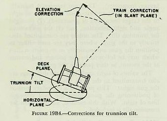
Figure 19B4 shows the necessary corrections. Applying the required correction by training left is training “uphill,” so that the bore axis would actually move above its original position. Therefore, it is necessary to depress the gun. It is evident that errors resulting from trunnion tilt cannot be corrected by applying equal and opposite amounts of gun train and elevation. Rather, it is necessary to compute the amount of movement in and perpendicular to the deck plane.

The mathematical solution of this problem is involved, and will not be included in this text. However, figure 19B5 shows how trunnion tilt corrections ensure that the gun will be offset from the LOS by Vs and Ds when the deck is inclined. The only practicable method of correction for trunnion tilt is by mechanical means, which will be discussed later.

19B14. Computation of gun orders

In modern gunnery, the gun battery is positioned to hit the target by training the guns to a certain angle relative to the fore-and-aft axis of the ship, and elevating them to a certain angle relative to the reference (deck) plane. These angles are known as gun train order and gun elevation order. Gun orders are computed mechanically in the range-keeper (computer). They are composed basically of (1) the bearing and elevation of the line of sight to the target (measured or generated), (2) the sight angle and sight deflection, and (3) the corrections for trunnion tilt. The orders are transmitted electrically to the guns, where they are used either to position the guns automatically or to position dials which may be followed by the pointer and trainer at the mount, as they position the guns.

The values of sight angle and sight deflection are also transmitted to the guns, where they are set on the gun sights. This provides a secondary method of positioning the guns, using the local telescope line of sight. With this method, no correction for trunnion tilt is included.

19B15. Correcting the fall of shot

Regardless of the accuracy of all computations, an error in the fall of shot may still exist. For example, information on which the calculations are based may not be completely accurate. These errors must be corrected by spotting the salvos to the target. The methods of spotting have been covered in the preceding chapter.

C. Graphic Rangekeeping

19C1. The Mark 2 plotting board

In the analytical solution (sec. 19B), target motion and own-ship motion in the LOS were calculated mathematically and combined into range rate. The same range rate may be determined by graphic analysis.

In 1911, the Mark 2 plotting board (fig. 19C1) was introduced and became an important part of the main-battery fire control system. In modern fire control systems the functions of the plotting board are performed by rangekeepers and their automatic graphic plotters. However, an explanation of the operation of the plotting board at this time will serve to demonstrate the fundamentals of all graphic rangekeeping.

The plotting board was designed to keep present range and to predict range for short intervals. It also provided a means of determining range rate and sight-bar range. It still is used to furnish a convenient method of keeping a time record of the firing, including deflection settings, spots applied, and times of salvos. This record is invaluable for post-firing analysis.

19C2. Principle of graphic plotting

If range is plotted against time, a series of points will be developed which may be connected to form a curve. If the points represent the mean of the ranges of several rangefinding instruments (as in fig. 19C2), the resulting curve is known as the mean range line. This is a graphic means of keeping the range.

Referring to figure 19C1, the range scale is moved downward at a fixed time rate. Ranges plotted along the range scale provide the points which are connected to form the mean range line. If ranging is interrupted for a short interval of time, the mean range line may be continued (or advanced) with little or no loss in accuracy. This has occurred from 3 minutes 10 seconds to 3 minutes 50 seconds in figure 19C2.

19C3. Range rate

An inspection of figure 19C2 reveals that if the mean range line slopes downward to the left, as in this case, the range is decreasing. The result is a decreasing or negative range rate. Conversely, if the mean range line were sloping downward to the right, the range rate would be increasing or positive.

The amount of slope at any point with respect to the time axis is a direct indication of the instant range rate at that time. More accurately stated, range rate varies directly as the tangent of the angle formed by a line tangent to the mean range line and the vertical (time axis). This is illustrated in figure 19C3.

Range rate determined in a similar manner on the graphic plotter of the modern rangekeeper is used to check the range rate generated by the rangekeeper. This will be explained in chapter 20.

19C4. Gun-range line

It is convenient to represent sight-bar range on the plotting board by means of a gun-range line, so named to distinguish it from the mean range line. Sight-bar range is the range shown on the sight scale of the gun at the instant of firing. It is the algebraic sum of present range, total ballistic correction, and range spots.

The total range ballistic correction may be calculated by means of a ballistic computation sheet. This ballistic correction is applied graphically to the mean range line on the plotting board. The result is the gun-range line, a second line which is drawn parallel to the mean range line. This gun-range line is offset as necessary whenever a spot is applied, and then continued parallel to the mean range line. The gun-range line furnishes sight-angle settings (in the form of sight-bar ranges) to the gun.

With this system there is of necessity a delay between the time the plotter decides to transmit a sight-bar range to the gun and the time the gun actually fires with this sight setting. The appropriate sight-bar range must be picked from the plot, transmitted to the gun, and set on the sights; and the gun must be fired. The period of time required for these actions is called dead time. This problem is solved by the plotter, who mentally advances the gun-range line by an amount equal to the dead time (determined by experience). He then picks off the sight-bar range corresponding to the time at which the guns will fire, and this value is transmitted to the guns.

It can be seen from the above discussion that the graphic solution of the fire-control problem is slow, difficult, and inexact in many ways. In the modern fire-control system, the graphic plot is used only as a check on the range rate generated by the rangekeeper.

D. Mechanical Solution — General

19D1. System elements

The principal components of a fire control system are the gun director, the computer (or rangekeeper), the stable element (or stable vertical) and the gun mount, with essential transmission and communications equipment. All these components are aligned upon installation, with the fundamental reference planes of the ship, and are maintained in proper alignment by frequent checks.

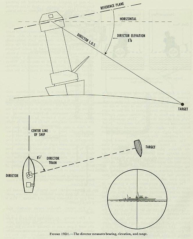
The gun director is located high in the ship’s structure, to get away from smoke and other interference and to provide as distant a horizon as practicable. The director may be rotated to any desired point in bearing, and the optical sights and radar antenna contained in it can be elevated within desired limits. By means of optical equipment and radar, the director is able to measure (1) the range to the target, (2) the relative bearing of the target, as an angle in the deck plane, measured clockwise from the bow, to the perpendicular plane through the line of sight, and (3) the elevation of the target as an angle above the deck plane. Ordinarily, the latter is measured by the stable vertical or stable element. The last two quantities are called director train and director elevation. In other words, the director establishes the line of sight to the target, and measures three aspects of the line of sight to form the basis of the problem: range, director train, and director elevation. These quantities are transmitted continuously to the computer. In addition, other values — chiefly estimated target speed and target angle — are transmitted from the director to the computer. (See figure 19D1.)

The computing instrument is located below decks. Its functions are to take the inputs from the director, plus additional information from other sources, such as own ship’s speed from the pitometer log, own ship’s course from the gyro compass, and the mechanical inputs from the stabilizing equipment; to combine these, computing the predicted position of the target and applying corrections; and to transmit the results to the guns as gun train order and gun elevation order.

The stabilizing equipment uses a gyroscope to measure the inclination of the deck plane with respect to the horizontal, resolves the deck tilt into components in and across the line of sight, and transmits this information to the computing instrument and to the director. (See figure 19D2.)

The gun is, of course, the striking force of the whole system. It is ordinarily equipped with automatic control equipment, including the necessary receivers to pick up the gun orders from the computer. The automatic control equipment points the guns by turning the whole mount in train and moving the guns themselves in elevation.

It may be helpful, in remembering the primary functions of the equipment, to think of the director as the eyes of the system, the computer as the brain, and the gun as the fist.

19D2. Reference systems

Since the fire control system is composed of many units installed at various places on the ship, sometimes at considerable distances both horizontally and vertically, it is necessary to install all the units in a consistent alignment and to make frequent checks to ascertain that proper alignment is maintained. The problem of establishing a reference system is covered in detail in chapter 21, Battery Alignment; the problem of correcting for horizontal and vertical displacement is treated in the next article. (See figure 19D3.)

19D3. Parallax

Figure 19D4 shows a typical installation with guns forward and aft and an amidships director. It shows that if a value of gun train order is based on the LOS from the director, a convergence correction is needed at the guns if they are to hit the target. This correction is called horizontal (or train) parallax, as it is caused by displacement in the horizontal and gives rise to an error in train.

If there is only one director, parallax does not enter into the value of director train. However, if there are two directors which are to be used interchangeably, as illustrated in figure 19D5, it is clear that the actual train angle of the two directors will differ by the amount of horizontal parallax. One director can be chosen as the reference point in train and the reading of the other director corrected to it, or a reference point can be chosen midway between the directors and the reading of both corrected to that reference.

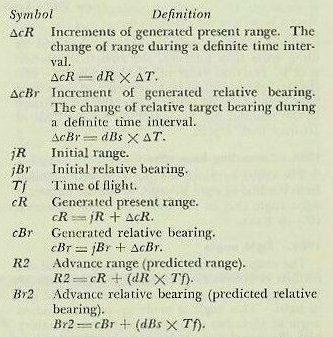
In computing horizontal parallax, it can be seen from figure 19D6 that the value depends on a number of factors:

1. The horizontal base length. The actual distance in the deck plane between the reference point and gun or reference point and director. This is a fixed quantity.

2. The range. Parallax varies inversely with range.

3. The bearing. In correcting both guns and directors for horizontal parallax, the quantity actually used is gun train or director train in the deck plane.

Mechanically, the quantity is multiplied by the reciprocal of range, which can easily be done, rather than divided by range, which is more difficult.

In some systems the computer works out the correction for a standard horizontal base length of 100 yards and transmits it to the guns. Gears at the gun or director in ratio of actual base length and standard base length are used to pick off the proper proportion of the correction. For instance, an element 50 yards from the reference point would need only half of the correction, as its own base length is half the standard. In other systems range, or a function of range, is sent to each gun and director, and similar corrections are worked out in computing devices located at each station.

Vertical parallax (Pv) depends on the range and the vertical displacement between the gun and the director.

E. Basic Mechanisms

19E1. Introduction

The study of any computer should be based on an understanding of the various basic mechanisms of which it is composed. These devices perform the mathematical computations essential to solution of the fire control problem. The present discussion will be limited to the most important basic mechanisms.

Mechanisms are represented by conventional symbols which facilitate their presentation on functional diagrams. Since the understanding of such diagrams is essential to the officer performing gunnery duties, these symbols are included in the figures depicting each mechanism.

19E2. Shafts

The computer receives inputs, performs computations, and transmits outputs. These quantities are in various units such as yards of range, degrees of elevation, knots of ship speed. Since, however, each of these quantities can be expressed as a number, it is possible to translate all quantities to shaft rotation. This procedure not only provides mechanical representation of the quantity; it also makes it easy to change or modify the quantity by suitable rotation. As the value of an input (such as own-ship speed) changes, the values of the computed quantities will change accordingly. These changes must be carried instantaneously and continuously to all the mechanisms affected by the change of input. These changing values are carried from one mechanism to another by shaft rotation.

Turning a shaft changes the value of the angle, speed, or distance represented by the position of that shaft. Rotation in one direction increases the value represented, and is considered positive; rotation in the other direction decreases the value, and is negative. From this, it follows that every shaft has a zero position, even though, as is sometimes true, the shaft may be restrained from reaching the zero position.

One revolution of a shaft can represent any convenient amount of change in the given quantity. For example, one revolution of the elevation shaft may represent a 3-degree change in elevation. On a range shaft, one turn may represent 100 yards of range. The value that a shaft carries in one revolution is called shaft value. Total value carried by a shaft is the shaft value multiplied by the number of revolutions made by the shaft from its zero position.

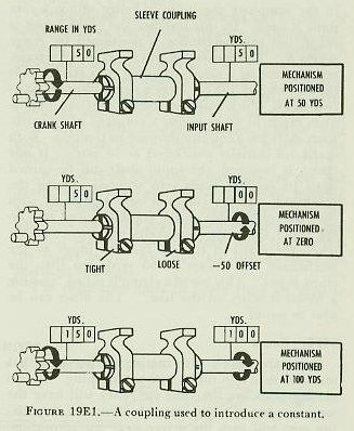
It is sometimes necessary to add or subtract a constant from a value carried by a shaft. For example, in the computer the value of range minus a constant is used. In this instance the crank input is range, but the mechanism is positioned for range minus K. The constant K can be set into the transmission line by a sleeve coupling or a clamp, as is shown in figure 19E1. Here a sleeve coupling joins two shafts which must introduce into the mechanism range in yards minus a constant of 50 yards. Each shaft has a counter showing its position. Both shafts are initially positioned at 50 yards. If one clamp is loosened, the input shaft can be turned until its counter reads zero without moving the crankshaft. If the clamp is now tightened, with the value of 50 yards on the crankshaft and zero on the input shaft, the two shafts will turn together when the crank is turned, but the input to the mechanism will always be 50 yards less than the crank input. This use of a clamp is called “putting a constant offset on the line.” The offset can be plus or minus.

19E3. Gears

Gears are wheels with mating teeth cut so that one can turn the other without slipping. If two mating gears are the same size, they will have the same number of teeth. One revolution of the driving gear will turn the driven gear one revolution, because each tooth of the driving gear will push one tooth of the driven gear across the line between their centers.

If two gears are of different sizes, the smaller is called a pinion, the larger a spur. When a spur gear and a pinion mesh together, their shafts turn at different speeds. If the spur gear has twice as many teeth as the pinion, one revolution of the driving gear will turn the pinion two revolutions.

The ratio between the number of teeth on the driving gear and the number of teeth on the driven gear is called the gear ratio. Gear ratios are often used for no other reason than to change the shaft values, by multiplication or division. If a shaft has a value of 500 yards per revolution, this can be reduced to 50 yards per revolution by a 1:10 gear ratio.

Although there are many different types of gears, most of those used in fire control installations are of three types: spur gears, bevel gears, and sector gears.

Spur gears are used to connect parallel shafts and transmit motion in opposite directions, as in figure 19E2.

Bevel gears can be designed to transmit motion between shafts at almost any angle to one another, as indicated in figure 19E3. By using bevel gears, several shafts at different angles can be driven by one driving shaft.

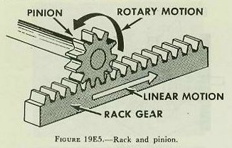
Sometimes only a part of a gear is needed, where the motion of the pinion is limited. In this case, space is saved by the use of a sector gear, illustrated in figure 19E4. A special type of sector gear is the rack, frequently used to convert rotary motion to linear motion. A rack is a straight bar with gear teeth cut in it, as shown in figure 19E5. If the rack drives a gear, it converts linear motion into rotary motion. The rack is restrained by guide rails which permit motion in one line only. The position of a rack indicates a value by the amount it has moved from zero.

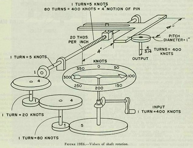
It must be understood that motion of a shaft, rack, gear, or dial has no meaning except that assigned by the designer. It is not difficult to design an assembly so that proper values are entered and transmitted. For example, the conversion constant 0.563, which converts knots to yards per second, is applied by a gear ratio. (A close approximation can be obtained by a gear ratio of 22:39, which equals 0.564.) The mechanism shown in figure 19E6 will serve to illustrate some of the principles presented in this section. The sequence starts with an input shaft, one turn of which represents 400 knots. The ratios of the gears have been designed to use the 4-inch motion of the rack, which is driven by a screw with 20 threads to the inch. Since each revolution of the screw shaft represents 5 knots, each inch the screw (and therefore the rack) moves equals 100 knots, and 4-inch travel of the rack represents 400 knots. It is possible to transform the output of the rack (linear motion) to shaft rotation as shown. If an output shaft carrying a gear with pitch diameter of 1 inch is used, one revolution of this output shaft will represent or 3.14 inches of linear motion of the rack. The value 4/3.14 turns of the output shaft will then represent 400 knots.

19E4. Differentials

A differential is a mechanism that can perform addition and subtraction. More precisely, it adds the total revolutions of two shafts or subtracts the total revolutions of one shaft from the total revolutions of another shaft, and delivers the answer by positioning a third shaft.

A differential will add or subtract any number of revolutions, or fractions of single revolutions, continuously and accurately. As inputs change, it produces a series of answers.

Figure 19E7 is a cut-away drawing of a bevel-gear differential, showing the relation of all its parts. Grouped around the center of a mechanism are four bevel gears, meshed together. These four gears and the spider shaft are the heart of the differential.

The two bevel gears on either side are the end gears; the two bevel gears above and below, meshing with the end gears, are the spider gears; the cross shaft and the spider gears constitute the spider, and the long shaft to which the cross shaft is pinned is the spider shaft. All gears are free to rotate on precision bearings.

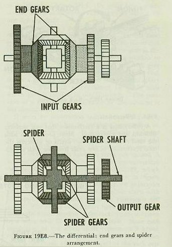
The three spur gears in figure 19E8 are used to connect the two end gears and the spider shaft to other mechanisms. They may be of any convenient size. The two attached to the end gears are normally input gears. An input gear and an end gear together make up a side of the differential.

The output gear is pinned to the spider shaft. It is the only gear in the mechanism that is pinned directly to a shaft.

Figure 19E9 shows how the spider gears work. The two end gears are positioned by the input shafts, which represent the quantities to be added or subtracted. The spider gears are driven by the two end gears, turning the spider shaft a number of revolutions proportional to the sum or the difference of the revolutions of the end gears.

Suppose the left side of the differential is rotated while the other is held stationary. The moving end gear will drive the spider gears, making them walk around the stationary end gear. This motion rotates the spider in the same direction as the input, and turns the output shaft with it. The output shaft will turn a number of revolutions proportional to the input.

If the right side is now rotated and the left side held stationary, the same thing will happen. If both sides of the differential are turned in the same direction at the same time, the spider will be turned by both at once. The output will be proportional to the sum of the two inputs. Actually, the spider makes only half as many revolutions as the sum of the revolutions of the end gears, because the spider gears are free to roll between the end gears. Of course, the answer can be corrected by using a 2:1 gear ratio between the output shaft and the next mechanism in the line.

When the two sides of the differential move in opposite directions, the output on the spider shaft is proportional to the difference of the revolutions of the two inputs. This is because the spider gears are free to turn, and are driven in opposite directions by the two inputs. If the two inputs are equal and opposite, the spider gears will turn, but there will be no movement of the spider shaft.

19E5. Cams

Gears can be used to convert one value to another when they are directly proportional. Differentials can add or subtract quantities represented by shaft rotation. However, in the fire control problem there are other functions which vary in a more complex manner. For example, drift and time of flight are functions of range, but not in direct proportion. Examination of the range table for the 5"/38 caliber gun will show that the value of drift for a range of 5,000 yards is 10 yards, but value of drift for 10,000 yards is 69 yards, considerably more than twice the value at 5,000 yards.

To obtain the correct mechanical output of drift for the values of range, a cam is used. A cam is a rotating or sliding device whose operating surface is cut to give the desired output for every value of input. The output is taken off by a cam follower. The follower may ride in a groove or slot in the cam face, or it may ride on the outside contour of the cam.

One simple cam has a uniform or constant-lead spiral groove cut in the face of a disc as shown in figure 19E10. Each point on the spiral corresponds to an output that is directly proportional to the input.

If the constant-lead cam is rotated in one direction, the spiral will force the follower block outward from the center along a straight slot. Turning the plate in the opposite direction forces the follower toward the center. The follower itself never travels to the center of the cam, but the output pin is offset on the follower block so that it can be positioned directly over the center of the cam for the zero position. The cam output is the distance from the center of the cam to the output pin, and can be picked off by a slide or rack. The output of the constant-lead cam is directly proportional to the input.

In other cams, each point on the output surface represents a more complex function, such as the reciprocal, the square, or some empirical function. Such cams are called computing cams to set them apart from the constant-lead type. Most cams used in computers are computing cams.

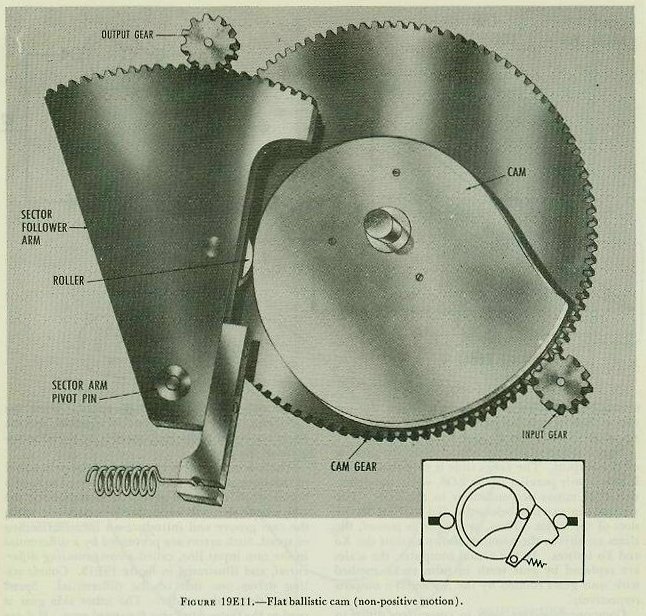
In the flat ballistic cam illustrated in figure 19E11, the edge of the cam does the computing. The cam is fixed to the cam gear and turns with it. A roller on the sector follower arm is held against the edge of the cam by a spring at the bottom of the arm. The distance from the center of the cam gear to the edge of the cam surface is designed to give the desired functional relationship. The movement of the roller pivots the sector arm which turns the output gear.

When the cam is so constructed that motion of the follower will positively result when the cam plate is moved, it is called a positive-motion type of cam. In the non-positive-motion type the follower is held against the cam surface by some acting force such as a spring or gravity. Figure 19E10 is an example of the positive-motion type, while figure 19E11 illustrates the other type.

19E6. Reducing cam displacement

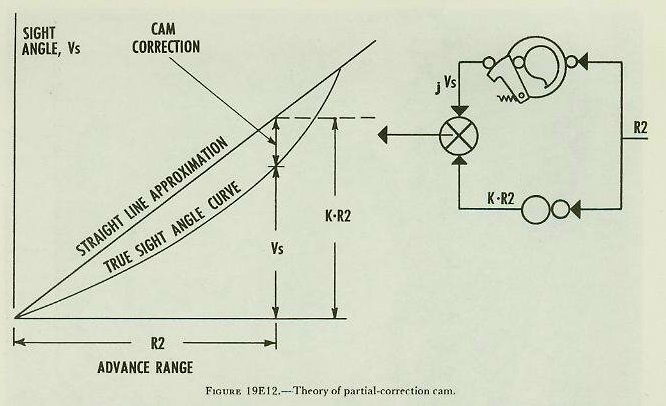
If a cam is cut to supply the full value of a function of a variable, it must necessarily be fairly large to provide accurate outputs. The size of the cam (and thus the ultimate size of the computer itself) can be greatly reduced if it is made to supply only a part of that function. This result can be obtained with the partial-correction cam which makes use of a straight-line approximation.

Assuming that it is desired to compute sight angle Vs by a cam, refer to figure 19E12. The true sight-angle curve is plotted in the figure with advance range R2 as the abscissa and sight angle Vs as the ordinate. A sample computation is represented graphically in the figure. At a given advance range R2, the corresponding sight angle Vs can be found from the graph by moving vertically from the value of advance range to the sight-angle curve. However, the actual cam is cut to produce not Vs, but the quantity labeled “cam correction” on the curve, jVs* on the diagram to the right. This correction is the difference between the true sight-angle curve and the straight-line approximation of the curve.

Since the straight line has constant slope, its ordinate at any given value of R2 is equal to a constant K times R2 (KR2). This multiplication can be accomplished by a gear ratio, as indicated.

The value of KR2 is then combined with the corresponding value of cam correction in a differential, as shown in the figure. The output of this differential will then be the value of Vs for the given R2. In other words, Vs = jVs + KR2. With this arrangement, the size of the cam is greatly reduced.

*The symbol j before a quantity, as used here, will be encountered frequently. As defined in the appendix, “Before a quantity it means a correction or partial correction to that quantity, usually generated by the mechanism; after the quantity it means an arbitrary correction (spot) to the quantity.” In mechanical computers, j is used before a quantity with two distinct meanings: first, as in present range (jR), in the sense of an initial or corrective setting; and second, as in the present case, the output of the partial-correction cam, where it expresses a partial value of the quantity — a value to which something else must be added to obtain the complete quantity.

19E7. Component solvers

The component solver is a device for resolving a vector into components with respect to a reference line. In the analytical solution of the fire control problem, it was shown that own ship, target, and wind motions are represented by vectors and resolved into components in and across the line of sight.

The component solver which resolves own ship’s motion into Yo and Xo is shown in figure 19E13. The dial carrying the compass rose and own-ship outline is free to rotate. The vertical pin may be moved in the radial slot. Two reference lines are shown, the vertical one representing the line of sight.

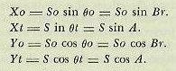
The center of the vertical pin corresponds to the arrowhead of a vector representing the motion of own ship. The distance of the pin from the center of the dial represents own-ship speed (So). The angular position of the radial slot with respect to the line of sight corresponds to relative target bearing. If Br and So are properly set, the displacement of the pin from the reference lines will be a measure of Xo and Yo to the same scale as that used for setting So, as shown in the small triangle. Inspection will show that the component solver solves the equations Xo = So sin Br and Yo = So cos Br.

Figure 19E13 shows the arrangement for picking off the outputs. The range slide is mounted so that it moves only parallel to the LOS, while the deflection slide moves perpendicular to the LOS. The vertical pin extends below the dial and fits in the slots of the slides. Thus, as the pin is moved, the slides are driven the amounts shown against the Xo and Yo indices. In the actual computer, the scales are replaced by gear teeth to form racks, meshed with spur gears rotated by the Xo and Yo outputs respectively.

Component solvers used in computers differ in details but operate according to the same principle. Figure 19E14 shows the type now in general use for resolution of ship, target, and wind motions.

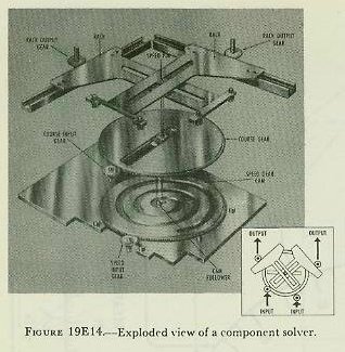
The dials indicating the speed and angle setting are on the face of the computer, separated from the actual component solvers but connected by suitable shafts and gears. The position of the course gear determines the direction of the vector with respect to the reference line. The radial position, or speed setting, of the pin is controlled by the spiral groove in the speed gear. When the speed gear is rotated with respect to the course gear, the spiral slot causes the pin to move in or out, setting the proper lengths of the vector representing ship’s speed. When the speed and course gears are rotated together, and the speed setting is unchanged, there is no radial movement of the pin.

There is one possible error in a component solver of this design. If the course gear is turned to reset a vector while the speed gear is held stationary, the course-gear slot will cause the pin to move along the cam groove and introduce an incorrect setting of speed. Such errors are prevented by a differential in the cam input line, called a compensating differential, and illustrated in figure 19E15. Course setting drives one side of the differential. Speed setting drives the spider. The other side gear is used as the output to drive the speed gear. If there is no speed input, the spider is held stationary, and the course input drives through the differential to turn the speed gear the same amount as the course gear, thus preventing any change in speed. If there is no motion of the course input, the speed input drives through the spider to turn the speed gear without disturbing the course gear. The differential thus causes the speed gear to be turned by both course and speed inputs, while the course gear is turned only by course inputs, so that correct settings of one can be made without introducing error into the other.

19E8. Integrators

Integrators, as used in computers, perform a special type of multiplication. In the disc-type integrator, illustrated in figure 19E16, a constantly changing value, such as time, is multiplied by a variable such as range rate, the output being a continuous value of their product which can be accumulated as shaft rotation.

The instrument consists of a flat circular disc revolved at constant speed by a motor equipped with a clock escapement; a carriage, containing two balls driven by friction with the surface of the disc, and themselves driving an output roller; and suitable shafts and gears for transmission of values to and from the unit. Rotation of the disc rotates the lower ball, which turns the upper ball, and this in turn rotates the output roller. The balls are supported in a movable carriage so that the point of contact between the lower ball and the disc can be shifted along a diameter from the center of the disc to either edge. Spring tension on the roller provides sufficient pressure to prevent slipping. Two balls are used to reduce the sliding friction that results when only one is used.

The speed of roller rotation depends upon the speed at which the balls rotate. If the carriage is in the center of the disc, no motion is imparted to the roller. As the carriage is moved off center, the balls will begin to rotate, and will reach their maximum speed at the edge of the disc. The speed varies with the distance of the carriage from the center. Values of rotation on one side of center are considered positive, while if the carriage is moved to the opposite side, rotation will be in the opposite direction and will give negative output values.

Figure 19E17 illustrates a practical application of the integrator to the solution of the fire control problem. It shows a simple situation in which a target at constant speed traveling a straight-line course passes own ship, which is stationary. Although target speed remains constant, the component along the line of sight, which is the whole range rate in this case, will gradually change from a negative rate through zero to a positive rate. The range rate continues to change, although speed is constant. The integrator solves such a problem with ease. The constant speed of the disc represents time, and the position of the carriage is set by range rate. The output of the roller then is generated range increments representing the sum of the products of time increments and range rate dR. These increments are added in a differential to the original setting of observed present range (jR) to give cR, generated present range.

19E9. Multipliers

In solving a fire control problem it is often necessary to multiply two continually changing values to produce a series of products. This is accomplished by a multiplier. Several types of multipliers are in use, all basing their solutions upon relationships existing between similar triangles. For reasons of space, it is convenient to build multipliers that deliver a fixed fraction of the answer, such as a tenth or a twelfth, rather than the complete numerical value required. The correct answer is supplied by suitable gearing.

Multipliers can take two continually changing input values and deliver an output that is proportional at every instant to the product of the two changing inputs.

The screw-type multiplier, illustrated in figure 19E18, has two inputs, which position a slide and a rack. The input rack is moved up and down by a spur gear. The input rack moves a slotted pivot arm that pivots around a stationary pin as the input rack is moved.

The multiplier pin is mounted in the slots of the input slide and the pivot arm where these slots cross. The position of this pin is changed by movement of the input slide or the input rack. The multiplier pin also fits into a slot in the output rack. As it changes position, the pin moves the output rack up or down.

The positions of the input slide and the input rack represent the two values to be multiplied together. The position of the output rack represents the output value, which is always proportional to the product of the two inputs.

Suppose the lead screws are turned until the multiplier pin lies directly over the stationary pin. This is the zero position of the input slide, since, with the slide in this position, movement of the input rack will not produce any movement of the output rack. This is shown in figure 19E19.

Similarly, if the slot in the pivot arm is positioned parallel to the slot in the output rack, no amount of motion of the input slide can cause any vertical motion of the multiplier pin or of the output rack. This is the zero position of the input rack.

Starting with both inputs at their zero position, suppose both input gears turn a few revolutions in the directions indicated. The input slide will move to the right. The input rack will move up its groove, bringing the pivot arm into an angular position. The multiplier pin will be pushed to its new position by the combined action of the pivot arm and the slide. This pin will move the output rack, and the output rack will turn the output gear.

Now, labeling the distances each part has traveled from the zero line: (1) the input rack has moved up a; (2) the input slide has moved over b; (3) the output rack has moved up x. If these distances are drawn on the diagram of the multiplier, they form two right triangles, as in figure 19E20. In the smaller triangle, the height, x, is the distance the output rack moved from zero. The base, b, is the distance the input slide moved from zero. In the larger triangle, the height, a, is the distance the input rack moved from zero. The base K is the fixed distance along the zero line from the stationary pin to the pivot on the input rack. Note that the two triangles are similar. It can now be seen that the ratio between the height and the base of the smaller triangle is equal to the ratio between the height and the base of the larger triangle.

That is: x/b = a/K. Multiplying both sides by b: x = ba/K.

This equation shows that the distance the output rack has moved from zero is equal to the product of the distances the input slide and rack have moved from zero, divided by a constant. In other words, the output is proportional to the product of the two inputs. Since K is a fixed distance, it is a constant value in each multiplier. Its effect is removed by proper choice of input and output gearing. Provision for both positive and negative x outputs can be made by placing the stationary pin at the center of the pivoted area.

F. Mechanical Solution — Basic Rangekeeper

19F1. General

The manner in which a computing instrument solves the surface fire control problem will be explained in this section, using the Rangekeeper Mark 8 as a model. This discussion is not to be considered a full presentation of the Rangekeeper Mark 8, which would be beyond the scope of this text; the student whose duties require more complete information is referred to the publications of the Bureau of Ordnance on the subject.

Figure 19F1 is a top view of the computing section of the Rangekeeper Mark 8, showing the arrangement of the various dial groups, knobs, and cranks. Figure 19F2 is a picture of the center dial groups, the upper dial indicating target course as well as wind direction; the lower dial showing own-ship course and target bearing. The line of sight from own ship to target is represented by the fixed indices, labeled “target bearing.” The dials thus give a visual picture of the own-ship and target set-up.

To clarify discussion, the rangekeeper may be considered to have three fundamental sections. This is a functional division of the rangekeeper rather than a physical one. The sections are: (1) The tracking section. (2) The prediction section. (3) The correction section.

19F2. Tracking section

The tracking section, given proper inputs, continuously provides the rates of change of range and bearing due to motion of own ship and target. It also generates present range, cR, and relative target bearing cBr. The target’s actual position relative to own ship is determined continuously by the director, which measures range and bearing. The generated values of range and bearing developed in the tracking section established a continuous value of present target position. When the rangekeeper is receiving the correct inputs, the actual target position and the generated position should be the same; this can be checked by comparing the actual and generated values of range and bearing.

19F3. Prediction section

Using values from the tracking section, the prediction section computes the position the target will occupy at the end of the time of flight. At the same time, this section computes the elevation and deflection offsets necessary to hit this predicted position in accordance with the range table and with existing variations from range-table standard conditions. The computation of these corrections is carried out in the ballistic part of the prediction section. The final step is to convert these predictions, including ballistics, into sight angle and sight deflection, the angular offsets from the line of sight which will position the gun to hit the target at the end of the time of flight.

19F4. Correction section

The correction section takes care of the effects of deck inclination. It has two parts, the trunnion-tilt corrector and the deck-tilt corrector. The trunnion-tilt corrector, as its name implies, corrects gun train and elevation for the tilting of the gun trunnions.

The deck-tilt corrector works out corrections to the line of sight to take care of deck inclination. The director measures the bearing of the target in the deck plane, but the computer works out its solution in the horizontal. Whenever the deck is tilted, these two values in the deck and horizontal planes will differ by the amount of the deck-tilt correction. The bearing in the horizontal plane is obtained by a differential which combines the bearing measured by the director with deck-tilt correction.

19F5. Rangekeeper computing mechanism

Having summarized in a few words the function of each major part of the rangekeeper, it will now be in order to return to each section of the instrument in turn for more detailed analysis. In the balance of this section of the chapter the intermediate quantities used in the development of gun orders will be considered as they are evolved from the original inputs to the computer. The ultimate purpose of the entire system is the computation of gun train order, B′gr, and gun elevation order E′g, the values which position the gun to hit the target.

19F6. Range rate, dR

The range rate, dR, is the algebraic sum of the components of own-ship and target motion in the line of sight: expressed in symbols, dR = Yo + Yt. The arrangement by which this is accomplished in the rangekeeper is shown in figure 19F3. Values of target angle, A, and target speed, S, (initially estimated by the spotter) are cranked into the target-component solver. The outputs of this component solver are the target components in and across the line of sight (Yt and Xt respectively).

Own ship’s speed, So, which is received automatically from the pitometer log, is combined in the own-ship component solver with an input of relative target bearing. (The generated rather than observed value of target bearing is used, for reasons which will be explained later.) The resulting outputs are the own-ship components in and across the line of sight (Yo and Xo respectively). The components in the line of sight, Yo and Yt, are then added algebraically in a differential, as shown in the figure, to obtain range rate, dR, expressed in knots. This quantity is next changed from knots to yards per second by means of a simple gear ratio. The value of dR also, through appropriate gearing, positions a counter on the face of the rangekeeper, and is used by the operator to compare with measured range rate and thus determine if correct set-up of the elements has been made.

19F7. Increments of generated range

If some means is provided to multiply the rate of change of range by time as it elapses, the result will be a continuous set of increments of range in yards. A disc integrator, previously described, accomplishes this. The value of dR is used to position the carriage of the range integrator; the disc is revolved by a constant speed time motor. The resulting output of the integrator is increments of generated range, which are constantly accumulated as shaft rotation.

19F8. Generated present range, cR

When the increments of generated range are added to the value of initial range, jR, as measured by the radar or rangefinder, the result will be generated present range, cR. Figure 19F3 shows how this is accomplished in the rangekeeper by means of a differential. The value of cR appears on a range counter on the face of the rangekeeper. It is also an important input to the prediction section.

19F9. Linear deflection rate, RdBs

Referring again to figure 19F3, it is seen that the deflection rate of the target, Xt, is an output of the target-component solver. The deflection rate of own ship, Xo, is provided by the own-ship component solver. These are added in a differential to produce the total linear deflection rate, RdBs. This is a linear rate in knots; it is then converted from knots to yards per second by means of a gear ratio.

19F10. Increments of bearing

It would be possible to compute linear increments of bearing in yards by multiplying RdBs by increments of elapsed time in an integrator, as was done in the case of increments of range. Since, however, an angular rather than a linear bearing rate is needed for the purpose of evolving generated bearing, it is necessary that a means be provided in the rangekeeper to convert linear increments of bearing, found as described above, to angular increments expressed in angular units, such as minutes of arc.

19F11. Increments of generated bearing

19F12. Generated bearing, cBr; regeneration

Generated bearing, cBr, is derived by integrating the angular bearing rate and adding the result to initial bearing jBr in a differential, as shown in the schematics above. The generated bearing cBr is then used to position the course gears of the own-ship and target-component solvers. This means that once the problem has been solved, this quantity drives back continuously to reposition the component solvers in accordance with the development of the relative-motion problem. This process is called regeneration, and is one of the most important features of the rangekeeper. Because of this regenerative feature, the rangekeeper is able to handle the indirect fire problem and, in fact, is able to continue to compute gun orders during any period when the director cannot see the target. Should the target change course or speed during such periods, of course inaccurate gun orders will result.

19F13. Summary of tracking section

The values supplied to the tracking section were (1) the known elements, So and Co; (2) the measured elements, jR and jB; and (3) the estimated elements, A and S. From these it has developed generated rates, dR and RdBs, and increments which have been used to determine the generated quantities cR and cB. Comparison of these generated values with the observed values transmitted from the director provides the rangekeeper operators with a method of checking the solution; i.e., of checking the estimates used for the values of A and S. This feature of operation, known as rate control, will be further developed in article 20E7 of the next chapter.

The outputs of the tracking section, dR, cR, and RdBs, become inputs to the prediction section, which makes use of them in the computation of sight angle and sight deflection.

19F14. Prediction of sight angle, Vs

Sight angle, as computed by the rangekeeper, includes the corrections for four quantities; namely, relative motion during time of flight, range wind, initial velocity loss, and a quantity known as range error due to deflection. Sight angle is computed in the vertical plane, and the assumption is made that the gun and target are in the same horizontal plane; that is, target elevation is assumed to be zero. Sight angle is merely the angular equivalent, in minutes of arc, of advance range in yards.

Advance range differs from the actual range to the advance position of the target by the ballistic corrections. To compensate for factors such as own-ship motion, target motion, wind, and variations in initial velocity, the gun must be elevated for a range equal to present range plus the algebraic sum of the several range compensations. During the time of flight, the target will travel to the computed point of fall shown, and the projectiles will hit. The equation for advance range is R2 = cR + Rj + Rtwmx.

Present range cR was generated in the tracking section. Rj, range spot, is entered into the rangekeeper as sent down from the director. It is now necessary to consider the several elements comprising Rtwmx and show how each is computed in the prediction section of the rangekeeper. The prediction Rtwmx is the sum of the following elements:

1. Rt — the range prediction to compensate for relative target motion during the time of flight, Tf. Relative target motion includes own-ship motion. It will be recalled that own-ship’s motion imparts additional velocity to the projectile, which is the effect here considered. Obviously any motion of own ship after the projectile leaves will have no effect on the projectile’s travel.

2. Rw — the range prediction to compensate for the effect of apparent wind on the projectile.

3. Rm — the range prediction to compensate for variations from the designed initial velocity.

4. Rx — the range prediction to compensate for the effect of deflection exclusive of drift.

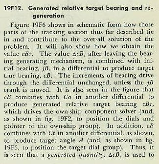
19F15. Range prediction, Rtw

The predictions to compensate for relative target motion and for wind are made in a multiplier called a range predictor (see fig. 19F7). If dR, the range rate, is multiplied by Tf, the result will be the relative motion in range during the time of flight. Since own-ship and target motion are added together to form dR, wind due to own ship’s motion must be handled separately. This is done by using apparent wind, a fictitious value which combines vectorially the true range wind and the range wind due to own ship’s motion. True-wind direction and velocity are set in the rangekeeper, the outputs of the wind-component solver being Yw and Xw, components of true-wind velocity in and across the LOS. Since apparent wind is the resultant of own-ship motion reversed and true-wind motion, range components of these elements are then combined in a differential, the output of which is Ywr, the component of apparent wind velocity along the line of sight (Ywr = Yo + Yw).

Instead of multiplying dR and Ywr by Tf separately, it is simpler to combine them and eliminate one multiplier. In computing Rtw (Rt + Rw), an empirical equation Rtw = Tf (dR − KYwr) + K1Ywr must be used, since Tf × Ywr alone will not produce the change in range caused by range wind (Ywr).

Referring again to figure 19F7, it is seen that range rate dR and apparent range wind Ywr are combined in a differential to give dR − KYwr, and this output is then multiplied by Tf to give jRtw, to which K1Ywr is added in a differential to give Rtw, the range prediction due to relative target motion and apparent range wind during the time of flight.

19F16. Range correction for I.V. loss and deflection exclusive of drift, Rmx

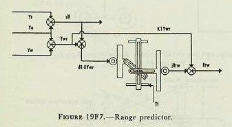
Referring to the schematic diagram of the prediction section, figure 19F10, it can be seen that Rtw, computed above, goes into a differential. Into the other side goes Rmx, the quantity now to be considered.

The correction Rm is easily understood, as it takes care of change in the initial velocity due to erosion or other causes. The setting is made by the initial-velocity knob and dial, which introduces jRm as shown in figure 19F9.

The need for correction Rx is not so apparent and can best be shown by a simplified example. In figure 19F8, own ship is shown to be motionless and the target is moving to the right from position 1 at the instant of firing to position 2 at the end of the time of flight. At position 1 target angle is assumed to be 90 degrees; range rate therefore is zero. It is also assumed for simplicity that there is no wind blowing and that the projectile leaves the guns at the design value of initial velocity.

Since dR is zero when the target is at position 1, the range prediction (Rt) will also equal zero and the value of advance range will be equal to present range. With the guns elevated for present range and deflected to compensate for the target’s rightward motion during the time of flight, it is obvious from the diagram that the salvo will fall short by the amount Rx.

This error is the result of computing the range prediction from an instantaneous value of dR which is based on the present line of sight; whereas dR will actually be a changing value if Br and A are changing during the time of flight. It will be noted that drift is excluded in the computation of Rx. The reason for this is that when the data for the various range tables are collected at the proving grounds, the range error caused by drift is compensated for.

From figure 19F9, it can be seen that drift, Df, is subtracted from total sight deflection, Ds, leaving Dtwj; that is, deflection exclusive of drift, and empirically jRx equals K (Dtwj)². jRx is added to jRm to give jRmx, which is one input to the range-correction multiplier, the other input being R2. The output is Rmx.

19F17. Total range correction, Rjtwmx

As shown in the schematic, figure 19F10, range prediction Rtw is now combined with range correction, Rmx, in a differential to give Rtwmx. Range spot, Rj, if any, is then combined with Rtwmx in another differential, the output of which is total range correction, Rjtwmx.

19F18. Advance range, R2

From the schematic, figure 19F10, it can be seen that advance range, R2, is obtained by adding the total range correction, Rjtwmx, to the present generated range, cR, driven in from the tracking section. It should be recalled that advance range, R2, is not equal to the actual range to the target’s predicted position, the difference being due to the ballistic corrections for I.V. loss, range correction due to deflection, wind, and range spots. These corrections are included to ensure that the gun will be elevated the proper amount to hit the predicted position.

Although R2 is a fictitious value and not the actual range to the target’s predicted position, when this range is converted into sight angle and applied at the guns, the result should be a gun elevation which will cause hits on the target.

As shown in the schematic, R2 is used for several purposes in the prediction section. The most important use is its conversion by means of a cam into its equivalent angular value, sight angle Vs, which is used in making up gun elevation order and for setting the sights at the guns. R2 is also a necessary input to the range-correction mechanism. R2 is also an example of regeneration — inspection of figure 19F10 shows that R2 is used to compute and correct itself; for example, it is used to compute Rmx, which becomes part of R2.

19F19. Sight angle, Vs

As mentioned above, R2 is used to compute sight angle Vs. Inspection of any range table will show that column 1 tabulates range in yards, while column 2 shows the corresponding sight angle. In the ballistic computer there are two sets of cams, one set for firing armor-piercing projectiles at full and at reduced velocities, and the other for firing high-capacity projectiles at full and at reduced velocities. Both sets are designed to function in accordance with this range-table relation. As shown on the schematic, R2 rotates the Vs cam and computes jVs, a partial correction, while R2 in a gear train computes KR2, the straight-line function. When combined in a differential, jVs + KR2 = Vs. This value is now ready to be used in making up gun-elevation order.

19F20. Prediction of sight deflection

The next step to be considered is the computation of sight deflection, Ds, the angular amount which the bore of the gun must be offset in the horizontal plane from the LOS. This quantity is made up of the following elements:

1. Dt — deflection prediction to compensate for relative target motion in deflection during the time of flight.

2. Dw — deflection prediction to compensate for the effect of apparent wind on the projectile during the time of flight.

3. Df — deflection prediction to compensate for drift.

4. Dj — manual deflection correction (spots).

19F21. Deflection prediction for relative motion, Dt

We have already studied the computation of RdBs, linear deflection rate due to relative motion of own ship and target, also the computation of advance range R2, and of Tf corresponding to advance range. If RdBs and Tf are multiplied, the result will be the linear deflection (in knots, which can be converted to yards per second by a gear ratio) due to own-ship and target motion.

When RdBs × Tf is known, the predicted position of the target at end of Tf is determined. However, to direct the guns, angular deflection from the LOS, Dt, is needed. In order to convert from linear to angular measure, advance range R2 must be considered, because the angular prediction varies with range and becomes larger as range decreases. The formula employed is:

Dt = 3,438 × RdBs × Tf / R2; in which Dt is in minutes, RdBs is in yards per second, Tf is in seconds, and R2 is in yards.

Reference to the schematic, figure 19F13, shows how the rangekeeper solves the above equation mechanically. The linear deflection rate RdBs, from the tracking section, is multiplied by Tf/R2 in the deflection-prediction multiplier to produce Dt. The constant K (3,438) is introduced by a gear ratio (not shown). After establishment of Dt, the angular prediction for relative motion, corrections must be made for wind and drift.

19F22. Correction for wind, Dw

Deflection prediction to compensate for the effect of apparent wind on the projectile, Dw, is computed in a multiplier known as the wind-deflection predictor. Xo (reversed) and Xw are added algebraically in a differential to give Xwr, the component of apparent wind velocity across the line of sight. This is multiplied by R2 to give Dw. Actually an empirical equation is used: Dw = (R2 − K1) Xwr.

The quantities Dw and Dt enter a differential to produce Dtw, as shown in figure 19F13. Deflection spot, Dj, if any, is applied by handcrank to make Dtwj. It will be recalled that Dtwj is used in the range correction mechanism to compute Rx, the range correction for deflection exclusive of drift.

19F23. Correction for drift, Df

The angular correction for drift increases as range increases; and, since this correction Df is very nearly proportional to advance range R2, Df is shown in the schematic, figure 19F13, as being produced by a gear ratio from an input of sight angle Vs. Df = (K − K1)Vs.

NOTE: Actually drift, Df, and Tf vary with R2 and are nearly proportional to Vs. In the rangekeeper the sight-angle cam output, Vs, after passing through suitable gearing, is used for Df and Tf/R2.

Df is added to Dtwj in a differential to produce sight deflection Ds; this value is now ready to be used in the computation of gun train order.

19F24. Summary of prediction section

The inputs to the prediction section were dR, cR, RdBs, Xwr, and Ywr from the tracking section as described previously, and a manual input of I.V. loss. In addition the prediction section receives any range and deflection spots which may have been made. The resultant outputs are Ds and Vs; these quantities are sent to the gun mounts for the purpose of setting the gun sights.

If it were not for the roll and pitch of the ship, gun orders could be made up simply by adding the computed values of sight angle and sight deflection to director elevation and director train:

E′g = E′b + Vs.

B′gr = B′r′ + Ds.

It will be noted that these equations not only assume a level deck, but also disregard corrections for parallax and roller-path inclination. This is justified by the fact that, in surface systems, the necessary corrections for these errors are made in instruments located at the directors and gun mounts, rather than in the rangekeeper.

Since the deck plane is rarely level, Vs and Ds, in addition to being used in computation of gun orders, must also be sent as inputs to the correction section, where with other values they form the basis of the correction necessitated by the inclination of the deck.

19F25. Level and crosslevel

Before considering in any detail how the two correctors in the correction section function, it is advisable to learn some of the details of the manner in which level and crosslevel are measured. Refer to figure 19F15. Level angle, L′, is measured about an axis in the deck; it is the angle between the horizontal plane and the deck plane, measured in the plane perpendicular to the deck through the line of sight. (This definition applies to level angle, L′, as measured in main-battery systems of battleships and cruisers which use the Rangekeeper Mark 8.)

As shown in figure 19F15, the line of sight is considered to be in the horizontal. Except for extremely short range, this assumption introduces no error. The deck plane is shown tilted with respect to the horizontal in such a direction that both level and crosslevel angles exist. By the definition of level angle (L′) above, L′ is measured in plane D — the plane perpendicular to the deck plane containing the line of sight — and it is the angle between the deck plane and the horizontal measured about an axis in the deck normal to plane D.

Crosslevel, Zh, is measured about the axis in the horizontal plane where the horizontal plane and the vertical plane containing the line of sight intersect; it is the angle between the vertical plane (plane A) and a plane perpendicular to the deck (plane D) through the axis just defined above.

19F26. The trunnion-tilt corrector

The trunnion-tilt corrector is installed in the Rangekeeper Mark 8 for the purpose of computing corrections to gun elevation order and to gun train order caused by the depression of one trunnion below the other. Referring to article 19B12, it will be recalled that, when the trunnion axis leaves the horizontal, the gun will elevate in a plane other than the vertical, and that the effective elevation above the horizontal will be less than Vs. A deflection error is also introduced, the effects of which are generally more serious than the elevation error. The trunnion-tilt corrector provides the necessary elevation correction Vz, and the train correction Dz, which are used in the rangekeeper as shown in figure 19F16.

The Stable Vertical Mark 41, which supplies the values L′ and Zh, will be taken up in the next section. The trunnion-tilt corrector computes Dz and Vz by solving the equations:

These equations are given merely to show the values entering into solution of Vz and Dz. They will not be further developed in this text, nor is it necessary to remember them.

19F27. Deck-tilt corrector

The function of the deck-tilt corrector is to correct B′r′, as measured in the deck plane, to a corresponding value of Br measured in the horizontal. Observed director train as received from a director must of necessity be measured in the plane of the director’s roller path, which is assumed here to be parallel to the reference plane. In order to compare generated target bearing, cBr, which is measured in the horizontal plane, with observed director train, B′r′, a correction, jB′r′, is added to the latter to convert it to bearing in the horizontal plane as shown in figure 19F16, thus changing it into observed target bearing, Br, in the horizontal plane. The deck-tilt corrector solves the equation:

The equation need not be memorized; it is given to show the student that the deck-tilt corrector requires inputs of B′r′, L′, and Zh.

19F28. Summary of correction section

The inputs to the correction section are Vs and Ds from the prediction section, and cB′r′ from the tracking section (the last used in place of B′r′ in the full regenerative set-up). B′r′ is received from the director; L′ and Zh are received from the stable vertical.

The output to the tracking section is jB′r′, which is therein combined with B′r′ to produce Br.

The other outputs of this section are (Vs + Vz) and Dd′ which equals (Ds + Dz). These quantities can now be used to compute gun orders which will be accurate with the deck tilted. The equations given in paragraph 19F24, when modified to obtain corrections for tilt, are as follows:

E′g = E′b + Vs + Vz.

B′gr = B′r′ + Dd′.

These expressions assume that the elements of the system are aligned to the reference plane, and that there is no parallax. Corrections for roller-path tilt and parallax are discussed in the next two articles, which summarize all quantities making up gun orders.

19F29. Gun elevation order

Gun elevation order is based on the elevation of the director pointer’s line of sight to the target, and is made up as shown in figure 19F18. This situation represents the most general case; that is, one which includes the most variables.

The director, when the sight is kept on the target, measures director elevation, E′b, which, with the deck inclined, includes level L′. E′b is corrected for vertical parallax and for director roller-path tilt to form the first element of gun elevation order, target position relative to the reference plane, measured from a reference point at the height of the gun.

Assuming for the moment that the gun roller path is parallel to the reference plane, all angles at the gun may be measured from the gun roller path, which represents zero gun elevation. Referring to figure 19F18, it can be seen that the angle level (L′) in effect reestablishes the horizontal plane. Measured below this is the angle E′, target elevation from the horizontal, which establishes a line of sight to the target from the reference point at the gun.

At this point the gun has received a signal which, when laid off from its roller path, gives a line of sight to the target. Now, if sight angle Vs is added to this signal, it can be seen in the figure that a gun position above the line of sight to account for predictions and ballistics is established. The gun-bore position above the line of sight must be corrected for trunnion tilt by the value Vz. The total angle of the bore axis above the roller path is gun elevation order, E′g. Since the roller path may not actually lie in the reference plane, the roller-path tilt corrector at the gun makes the necessary correction for this discrepancy.

Figure 19F19 is a diagram of the director, rangekeeper, stable vertical, and guns, in which the origin of the various quantities is shown. These quantities are actually combined within the rangekeeper, but they have been shown outside for clarity.

19F30. Gun train order

Gun train order is shown diagrammatically in figure 19F20. Director train, B′r′, establishes the target position relative to ship’s centerline, measured in the deck plane. A non-reference director will include a horizontal parallax connector, which will cause the director to transmit director train for parallax, which in effect establishes a line of sight from the reference point. This gives present position of the target relative to ship’s centerline and in the deck plane.

Measured from the fictitious line of sight from the reference point, sight deflection, Ds, is applied to account for predictions and ballistics, as can be seen in figure 19F20. Ds is computed in the horizontal plane, but if crosslevel is present the trunnion-tilt train correction, Dz, is added to produce the computed line of fire from the reference point. The sum of these angles is the angle that the computed line of fire makes with own ship’s centerline; that is, gun-train order, B′gr, in the deck plane. Gun train order is transmitted to the guns, where the proper horizontal parallax correction is applied to produce actual gun train to hit the target.

Figure 19F21 is a diagram of the gun train system. As shown in figure 19F21, director train, B′r′ corrected for horizontal parallax, is received by the rangekeeper. It also is transmitted to the stable vertical to keep the gimbals oriented with the line of sight, so that the stable vertical can measure the values of level and crosslevel in the proper planes.

The prediction section computes sight deflection, Ds, in the horizontal plane, to account for relative motion and deflection ballistics. The train correction, Dz, for trunnion tilt is computed in the trunnion-tilt corrector. This value accounts for the effect of crosslevel on the gun bore. Dz is added to Ds to produce deck deflection, Dd′, and this in turn is added to B′r′ to produce gun train order, B′gr, in the deck plane, which is then corrected for horizontal parallax at each gun.

G. Mechanical Solution — Establishing the Horizontal Plane

19G1. Introduction

Guns are installed with their roller paths parallel to the deck plane, so that their movement is limited to train in the deck plane and elevation above the deck plane. On the other hand, Vs and Ds are computed with reference to the horizontal. Since the deck plane of a moving ship deviates from the horizontal by the amount of roll and pitch, some means must be found to measure and correct for this discrepancy. Correction for deck inclination is most satisfactorily applied in the solution of the fire control problem if it is resolved into components in planes in and across the line of sight. The component in the line of sight, called level, then becomes a modification to elevation; while the component across the line of sight, called crosslevel, affects both train and elevation, as it causes the trunnions of the guns to tilt.

In early director systems the pointer’s telescope established the line of sight and a crosslevel telescope at right angles to it was kept on the horizon. The amount these telescopes had to be elevated or depressed from their zero position measured the tilt of the deck, and was applied as a correction within the rangekeeper. This method is used as a standby procedure in one modern system. It is fairly satisfactory, but is subject to human error, and is useless when the horizon is not visible.

Modern surface systems use, as their primary method of measuring level and crosslevel, an instrument called a stable vertical, which is essentially a gyroscope equipped with suitable mechanical and electrical pick-offs. The instrument establishes and maintains the true vertical and its associated horizontal plane, continuously measures level and cross-level, and transmits these values mechanically and electrically to the Mark 8 rangekeeper.

19G2. Gyroscopic principles

To understand the action of the stable vertical, it is necessary to understand the principles of the gyroscope. Any rapidly spinning mass will show the characteristic properties of a gyroscope. But for simplicity this discussion will be confined to a wheel, spinning rapidly on its axis.

A rapidly spinning wheel shows two properties that make it especially useful in fire control instruments. One of these properties is rigidity in space. This means simply that a wheel, as long as it is spinning rapidly, tends to keep its axis pointed in the same direction in space. (Because the earth itself is spinning, the wheel will not necessarily tend to keep its axis pointed in the same direction with respect to the earth’s surface. This is explained in article 19G4.)

A spinning top shows a good example of gyroscopic action. When it spins at high speed, the top remains erect, keeping its axis vertical. As the speed dies down, the axis is no longer able to maintain a fixed direction in space; the top begins to wobble, and eventually falls over. A bicycle wheel is another familiar example. Because of gyroscopic action, a bicycle is more easily balanced at high speed than when it is moving slowly.

Another name for the principle of “rigidity in space” is gyroscopic inertia. The inertia of the spinning wheel is the cause of its gyroscopic action. To understand this, consider the effect of inertia on any point on the wheel’s rim. The law of inertia states that when any body is in motion, it will continue indefinitely to move in a straight line, at the same speed, unless acted on by some external force. Any point on a spinning wheel is moving in a circular path. Because of its inertia, such a point will tend to move in a straight line, tangent to its circular path. But molecular attraction within the wheel tends to hold the particles together, and at normal speeds will confine all particles in the wheel to circular paths. The inertia of all the particles in the wheel, then, will tend to keep these particles moving in circular paths, with the result that the wheel tends to keep spinning in a single plane, and its axis tends to point in a single direction. The wheel will maintain its plane of rotation, and the axis will maintain its fixed direction, until the system is acted on by some outside force.

The inertia of a spinning wheel, and therefore the reliability of its gyroscopic action, depends on two things: the mass of the wheel, and the speed with which it is moving. For that reason, a gyroscope is relatively heavy, and is rotated at high speed. The speed of any particle on the gyroscope wheel depends not only on the speed of rotation, but also on the distance of the particle from the center. For that reason the weight of a gyroscope wheel is usually concentrated in its rim.

Another useful property of a gyroscope is precession. This term refers to the manner in which a gyroscope responds to any force that tends to change its plane of rotation, or the direction of its axis. When the speed of a spinning top decreases, gravity tends to pull the top down, and turn its axis horizontal. The top responds to the force of gravity by moving its axis at a right angle to the applied force. The resulting wobble is an example of precession.

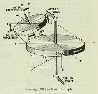
A study of figure 19G1 will show that precession, like rigidity in space, is a result of inertia. Imagine that the larger wheel in the figure is spinning rapidly. If a force is applied that tends to change the direction of the axis — represented by the two arrows marked “applied force” — the wheel responds to the applied force by precessing — by moving its axis in a direction at 90 degrees from that of the applied force.

To understand this action, consider the forces acting on point A at the instant represented by figure 19G1. The inertia of this moving point tends to carry it in the direction AC. The applied force tends to move point A in the direction AB. The point A responds to the two forces by moving in the resultant direction AD. This direction and length represents the vector sum of the two forces acting on point A. Point A can move in the direction AD only by turning the wheel’s plane of rotation to the position shown in the smaller diagram.

Precession, then, results in a movement of the axis in a direction at 90° from that of the applied force. As a result of precession, the axis of rotation (X-X), tends to become parallel to the axis of torque (Y-Y). Precession will continue until the applied force is removed. Inspection of figure 19G2 will provide a ready means of determining direction of precession. If a downward force is exerted on the gyro case as shown (at north) a gyro rotating clockwise will precess in the direction indicated (to the east).

Since level and crosslevel are angles measured between the reference plane and the true horizontal, the stable vertical accomplishes this measurement by containing a free gyro mounted inside an instrument case. The case itself is bolted to the deck in such a way as to be exactly parallel to the reference plane. Then, with the gyro maintaining its spin in the horizontal, the differences between the position of the gyro and the reference plane are measured and applied as needed.

19G3. Righting system

The gyro wheel is made to assume a horizontal position while spinning, and to maintain its original plane of rotation, by means of a mercury control system which opposes any external force tending to displace it.

Essentially the mercury control system consists of two tanks containing mercury, attached to the casing which houses the gyro wheel, on diametrically opposite sides of the wheel. These two tanks are joined by a narrow connecting tube, so that mercury is free to flow from one tank to the other. As long as the gyro wheel is exactly horizontal, the mercury level in both tanks will be the same; but as soon as the wheel is tilted from the horizontal by some external force, gravity will cause mercury to flow from the high tank to the low tank. The additional mercury in the low tank will then produce the same effect as a downward pressure exerted at the low point of the gyro wheel. Application of the rule of precession (fig. 19G2) shows that this will only cause the wheel to precess more out of the horizontal in a direction 90° away. However, if the mercury effect is applied not at the low point but 90° from the low point, pressure at this point causes the low point of the gyro to precess upward to its original horizontal position, at which point the mercury is redistributed equally.

This effect is accomplished in the stable vertical by rotating the entire gyro assembly and attached mercury tanks at 18 rpm in the same direction as gyro spin, and by restricting the size of the orifice to regulate the flow of mercury in the connecting tube. The net result is that by the time the mercury has reached the low tank, the low tank has been displaced 90° from the low point of the gyro wheel, and the pressure exerted here causes the gyro spin axis to precess back into the vertical.

It should now be apparent that when the gyro is first started, exactly the same action takes place to cause the gyro spin axis automatically to erect itself and settle in the vertical, after several minutes of operation.

19G4. Effect of the earth’s rotation

Further consideration will indicate that the horizontal plane necessary for purposes of fire control is a plane tangent to the earth’s surface at the ship’s position. A gyroscope originally set in this plane will not remain in the horizontal, as the earth rotates, unless some means is provided to compensate for the effect of earth’s rotation.

A gyro located at either pole will be unaffected, as the plane tangent to the earth at these points remains fixed in space. On the other hand, a gyro located at the equator will assume the successive positions with respect to the earth shown in figure 19G3 (A). To an observer standing on the earth, the wheel will turn completely over every 12 hours; that is, turn backward with respect to the earth’s rotation at the rate of one revolution in 24 hours.

At any point between the pole and the equator, as shown in figure 19G3 (B), the wheel gyrates once every 24 hours about an axis parallel to the axis of the earth’s rotation and in a direction opposite to that of earth’s rotation.

This effect can be compensated for if the gyro can be made to precess slowly to the eastward at the same rate as the earth’s rotation. The gyro’s plane of rotation will then remain parallel to the horizontal plane. This is accomplished in the stable vertical by means of a latitude weight which is so arranged that the effect of the weight is to cause a downward pressure at the north point of the gyro wheel, resulting in an easterly precession. The position of the latitude weight is adjustable, so that it can be set for the latitude in which the ship is operating.

Actually, the mercury control system would tend to keep the gyro spin axis vertical, but if the mercury control were acting alone, the gyro would still tend to deviate slightly from the vertical as a result of the apparent precession caused by the earth’s rotation. The latitude weight compensates for this error.

19G5. Mechanical construction

The Mark 41 stable vertical consists essentially of a sensitive element and a measuring group. The sensitive element is the heart of the instrument and consists of the gyro, gyro case, gyro gimbal, and a fork-shaped support known as the rotating fork.

Figure 19G4 shows the gyro proper. The wheel is carried on an axle supported by ball bearings at the upper and lower ends of the gyro case, the wheel and case forming the rotor and stator of a high-frequency induction motor. The squirrel-cage winding, consisting of solid conducting bars, is in the gyro wheel, while the wire stator windings are in the gyro case. A special motor-generator is provided to supply power at a frequency sufficient to drive the gyro at about 8,500 revolutions per minute.

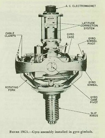
The gyro assembly of figure 19G4 pivots within the gyro gimbal on a case axis perpendicular to the spin axis, as shown in figure 19G5. The gimbal ring, in turn, is supported by the arms of the rotating fork on the gimbal axis, which is perpendicular to both the case axis and the spin axis. This axis arrangement provides a universal mounting giving the gyro three degrees of freedom, and allows it to spin on a vertical axis, even though the rotating fork may vary its inclination from time to time.

The measuring group consists of a level gimbal, a crosslevel gimbal, and a training gear. Figure 19G6 shows the arrangement of the measuring gimbals. The outer gimbal is the level gimbal, supported at its trunnion bearings by the training-gear structure (main frame). The level gimbal, in turn, supports the inner or crosslevel gimbal, so that its axis is perpendicular to the level-gimbal axis. At the lower end of the crosslevel gimbal the bearing for the rotating fork can be seen.

The entire sensitive-element assembly of figure 19G5 is mounted within the measuring-gimbal system of figure 19G6, being supported at its lower end by the rotating fork in its fork bearing, so that it is free to rotate within the measuring group. The complete assembly is shown in figure 19G7. A gimbal rotation motor, attached to the lower end of the crosslevel gimbal, is geared to the rotating fork and drives it at about 18 revolutions per minute. The fork turns the entire sensitive element at this speed within the measuring-gimbal system. This rotation is essential to the mercury control system.

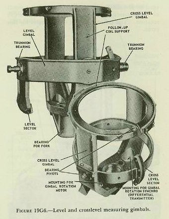
19G6. Director train input

Since level and crosslevel angles must be measured with respect to the LOS, director train B′r′ is received at the stable vertical to position the training gear. The training gear carries with it the main frame, which in turn supports the measuring group and the sensitive element. In this manner, the instrument is so oriented that the crosslevel axis lies in the direction of the LOS, with the level axis perpendicular to the LOS. Level, then, is measured in the LOS, and crosslevel 90° from the LOS.

Since the level gimbal axis is supported by the main frame, it lies in the deck plane, and level angle L′ as measured by this gimbal, is measured in a plane perpendicular to the deck plane. On the other hand, the crosslevel gimbal is so mounted that it remains in the horizontal and measures cross-level angle (Zh) in a vertical plane. These features of construction cause the stable vertical to measure L′ and Zh in accordance with the definitions of article 19F25.

19G7. The follow-up system

The actual measurement of L′ and Zh is accomplished by an electrical follow-up system. Figure 19G5 shows an electromagnet installed at the upper end of the gyro spin axis. This magnet remains in the true vertical because of the action of the gyro. Above the magnet but attached to the top of the crosslevel gimbal is an umbrella containing two figure-eight follow-up coils at right angles to each other, one for level and the other for crosslevel.

Roll or pitch of the ship will cause movement of the umbrella with respect to the magnet, inducing voltages in the follow-up coils by transformer action. The voltages so induced are amplified and rectified at a stable-vertical control panel, and are then used to energize level and crosslevel follow-up motors, which drive back through the gear trains, causing the level and crosslevel gimbals to move.

When the umbrella is back in its neutral position over the electromagnet, voltages are no longer induced in the coils and the follow-up motors cease to drive.

The follow-up coils are so constructed that they pick off voltages proportional to L′ and Zh, respectively. The amount of rotation of the follow-up motors necessary to cause the gimbals to maintain the umbrella at the neutral point over the electromagnet is then a direct measure of level and cross-level. These outputs are transmitted electrically and mechanically to the instruments requiring these values.

The response of the follow-up system is made sufficiently sensitive to cause the umbrella center to remain very nearly in line with the magnet. The motors drive practically as soon as displacement begins, so that the measurement of L′ and Zh is continuous and almost instantaneous.

An anti-hunt unit is installed at the control panel, and operates to shut off the power to the motors slightly before the neutral position is reached, preventing the umbrella from over-running the neutral position and driving back toward it again.

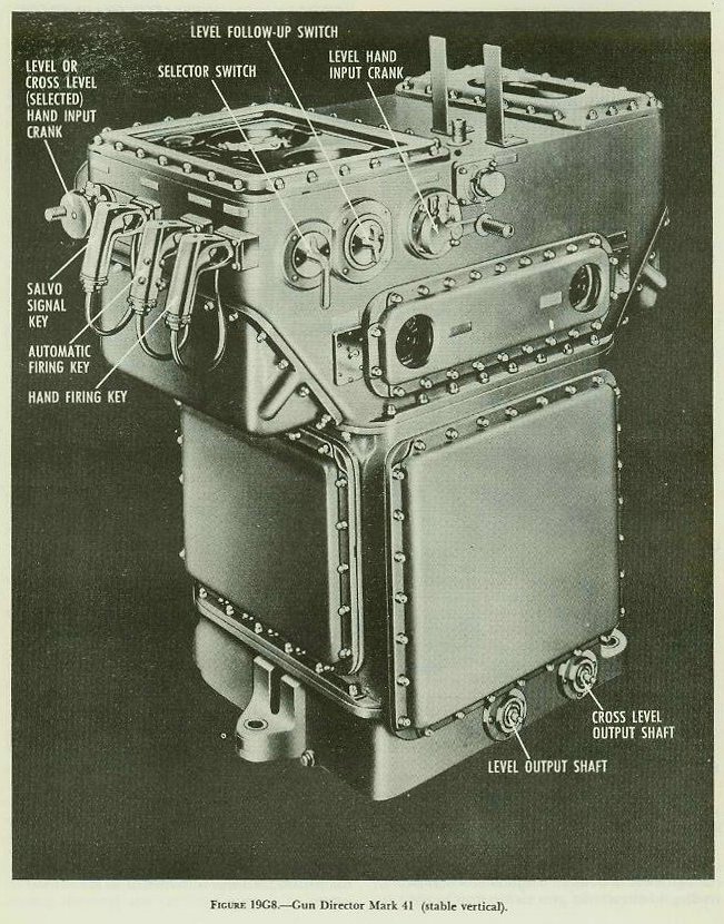
19G8. Mercury cut-out valves

The mercury control system has already been described. It normally operates to keep the gyro axis in the vertical. At times, however, certain irregularities of ship motion, such as sharp turns and speed changes, occur which would cause an irregular flow of mercury, tending to disturb the gyro rather than to right it.

To prevent mercury flow at such times, a mercury cut-out valve closes, blocking the connecting tube. This valve is operated automatically by a cut-out control on the control panel. During starting, the valve should remain open and therefore is made inoperative, since ship motion has no appreciable effect on the settling of the gyro. After the gyro has settled, the valve is connected to the automatic control.

19G9. Latitude motor input

It will be recalled that the latitude weight must always apply its downward force at the north point of the gyro wheel, and that the amount of force must be varied in accordance with the ship’s distance from the equator. This is accomplished by manually moving the latitude weight inward or outward in its mounting. It is usually considered sufficient to make a latitude setting once a day.

The sensitive element continuously rotates at 18 rpm, and the entire assembly is oriented to the LOS by B′r′. Since the latitude weight is mounted at the upper end of the gyro spin axis as shown in figure 19G5, provision must be made to cancel out the effects of the rotation and the B′r′ input. This is done by mounting the latitude weight on the rotor of a synchro known as the latitude motor. The stator rotates in accordance with the inputs of 18 rpm and B′r′, but the rotor carrying the latitude weight is positioned by a signal impressed on the windings of the stator. This input signal is made up of Co + B′r′ − 18 rpm, with the result that the rotor keeps the weight positioned in the north-south plane.

The input is obtained by combining the stable-vertical inputs of Co and B′r′ in a differential generator to get an output of Co + B′r′. This output is then combined in a second differential generator with 18 rpm from the gimbal-rotation motor, to give Co + B′r′ − 18 rpm, which is used as the input to the latitude-motor stator.

19G10. Manual follow-up

The L′ and Zh follow-up motors normally keep the umbrella positioned automatically over the gyro axis. Usually, then, the level and crosslevel hand input cranks are disengaged and the L′ and Zh follow-up switches are set at AUTOMATIC. Should either follow-up motor fail, the appropriate follow-up switch is set at MANUAL and its associated hand crank is engaged. This action breaks the circuits to the follow-up motor and transfers the umbrella’s pick-off signal from the amplifier unit to the galvanometer shown on the face of the instrument. The hand crank is then turned, to reposition the gimbal and umbrella over the magnet by keeping the galvanometer needle as nearly as possible in its zero position. Manual follow-up can be used instead of either or both follow-up motors.